Note:
GPRsurvey
However, this tutorial will not explain you the math/algorithms behind the different processing methods.
I suggest to organise your files and directories as follows:
/2014_04_25_frenke
    /processing      (here you will save the processed GPR files)
    /rawGPR          (the raw GPR data, never modify them!)
    /coord           (coordinates data)
        /FID         (fiducial marker files)
        /FIDmod      (modified fiducial marker files)
        /shapefiles  (here you will export the coordinate shapefiles)
        /topo        (ASCII files containing the trace coordinates)
    measured_coordinates.txt  (the topographic field measurements)
    RGPR_tutorial.R           (this is you R script for this tutorial)
Load the packages RGPR and rChoiceDialogs (rChoiceDialogs provides
a collection of portable choice dialog widgets):
library(RGPR)   # load RGPR in the current R session
library(rChoiceDialogs)
[optionally] If RGPR is not installed, follow the instructions of
the tutorial “Getting started” to install it.[optionally] If R
answers you there is no package called 'rChoiceDialogs' you need first
to install rChoiceDialogs, either through your R software or directly
in R with:
install.packages("rChoiceDialogs")
The warnings that R shows can be ignored.
The working directory must be correctly set to use relative filepath. The working directory can be set either in your R-software or in R directly with (of course you need to change the filepath shown below):
myDir <- file.path(c("/media/huber/Elements/UNIBAS/software/codeR",
                     "package_RGPR/RGPR-gh-pages/2014_04_25_frenke"))
setwd(myDir)    # set the working directory
getwd()         # Return the current working directory (just to check)
[optionally] Alternatively, you can use an interactive dialog box from
the R-package rChoiceDialogs:
myDir <- rchoose.dir(default = "/home/huber/WORK/UNIBAS/RESEARCH/RGPR/")
setwd(myDir)    # set the working directory
getwd()         # Return the current working directory (just to check)
GPRsurveyAn object of the class GPRsurvey is like an index that contains some
of the meta-data of several GPR data recorded during one survey. With
the class GPRsurvey you have an overview of all your data, you can
compute the positions of the profile intersections, plot a top view of
the survey and plot the data in 3D with open-GL (implemented in the
R-package RGL).
Read all the GPR records (“.DT1”) located in the directory /rawGPR
with the exception of the file CMP.DT1 and create an object of the
class GPRsurvey. To indicate the filepaths of the GPR data to R you
have the following options:
use a dialogue window
# select all the GPR files except CMP.DT1
LINES <- rchoose.files(caption = " DT1 files", filters = c("dt1","*.dt1"))
write manually all the filepath in a list
# select all the GPR files except CMP.DT1
LINES <- c()    # initialisation
LINES[1] <- file.path(getwd(), "rawGPR/LINE00.DT1")
LINES[2] <- file.path(getwd(), "rawGPR/LINE01.DT1")
LINES[3] <- file.path(getwd(), "rawGPR/LINE02.DT1")
LINES[4] <- file.path(getwd(), "rawGPR/LINE03.DT1")
LINES[5] <- file.path(getwd(), "rawGPR/LINE04.DT1")
take advantages of vectorized code
LINES <- file.path(getwd(), "rawGPR",
                   paste0("LINE", sprintf("%02d", 0:4),".DT1"))
extract automatically all the GPR file from the directory
# list of the filepath
allFilesinDir <- list.files(file.path(getwd(), "rawGPR"))
allFilesinDir
##  [1] "CMP.DT1"    "CMP.HD"     "LINE00.DT1" "LINE00.HD"  "LINE01.DT1"
##  [6] "LINE01.HD"  "LINE02.DT1" "LINE02.HD"  "LINE03.DT1" "LINE03.HD"
## [11] "LINE04.DT1" "LINE04.HD"
# now, select only the file ending with.DT1 and without "CMP"
# in their names
selDT1 <- grepl("(.DT1)$", allFilesinDir, ignore.case = TRUE) &
!grepl("CMP", allFilesinDir, ignore.case = TRUE)
LINES <- file.path(getwd(), "rawGPR", allFilesinDir[selDT1])
same as above but shorter!
list.files(file.path(getwd(), "rawGPR"), pattern = "LINE[0-9]+\\.DT1")
## [1] "LINE00.DT1" "LINE01.DT1" "LINE02.DT1" "LINE03.DT1" "LINE04.DT1"
GPRsurveymySurvey <- GPRsurvey(LINES)
Have a look at the newly created object:
mySurvey
## *** Class GPRsurvey ***
## Unique directory: /mnt/data/Documents/RESEARCH/PROJECTS/RGPR/CODE/RGPR-gh-pages/2014_04_25_frenke/rawGPR
## - - - - - - - - - - - - - - -
##     name length units       date freq coord int   filename
## 1 LINE00    56.     m 2014-04-25  100    NO  NO LINE00.DT1
## 2 LINE01    12.     m 2014-04-25  100    NO  NO LINE01.DT1
## 3 LINE02    69.     m 2014-04-25  100    NO  NO LINE02.DT1
## 4 LINE03    90.     m 2014-04-25  100    NO  NO LINE03.DT1
## 5 LINE04   111.     m 2014-04-25  100    NO  NO LINE04.DT1
## ****************
You can see that no coordinates (x,y,z) are associated with the GPR data. Therefore, if you try to plot the survey you will get:
plot(mySurvey, asp = 1) # throw an error
Note that the object mySurvey only contains the meta-data and a link
to the GPR files (that are stored in your working directory). But
mySurvey does not contains the GPR data itself (i.e. the traces).
However, we can ask mySurvey to read the data and return it in the
form of an object of the class GPR. There are two possibilities:
Either subset mySurvey with [[ ]]
A02 <- mySurvey[[3]]
A02
## *** Class GPR ***
##  name        = LINE02
##  filepath    = /mnt/data/Documents/RESEARCH/PROJECTS/RGPR/CODE/RGPR-gh-pages/2014_04_25_frenke/rawGPR/LINE02.DT1
##  description =
##  survey date = 2014-04-25
##  Reflection, 100 MHz, Window length = 399.6 ns, dz = 0.4 ns
##  275 traces, 68.5 m
##  ****************
Or get the GPR object with the function getGPR()
A02 <- getGPR(mySurvey, id = "LINE02")
A02
## *** Class GPR ***
##  name        = LINE02
##  filepath    = /mnt/data/Documents/RESEARCH/PROJECTS/RGPR/CODE/RGPR-gh-pages/2014_04_25_frenke/rawGPR/LINE02.DT1
##  description =
##  survey date = 2014-04-25
##  Reflection, 100 MHz, Window length = 399.6 ns, dz = 0.4 ns
##  275 traces, 68.5 m
##  ****************
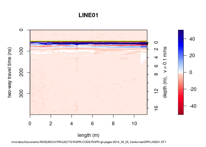
You can also directly plot the GPR data with:
# instead of 'A02 <- mySurvey[[3]]' and 'plot(A02)' do:
plot(mySurvey[[2]])
There are two options: (1) either you already have the coordinates of each traces or (2) you have the coordinates of points that were marked in the GPR data using fiducial marker.
We assume that for each GPR record there is a file containing the (x, y, z) coordinates of every traces. The header of these files is “E”, “N”, “Z” instead of “x”, “y”, “z” because in topography “x” sometimes designates the North (“N”) and not the East (“E”) as we would expect. The designation “E”, “N”, “Z” is less prone to confusion and therefore we chose it!
Define the filepaths to the topo files:
# select all the GPR files except CMP.DT1
TOPO <- file.path(getwd(), "coord", "topo",
                  paste0("LINE", sprintf("%02d", 0:4), ".txt"))
Read all the ASCII files with the function readTopo() that creates
a list that contains the coordinates of every traces (readTopo()
will automatically detect the column separator as well as the
presence of header in the ASCII files):
TOPOList <- readTopo(TOPO)
## read /mnt/data/Documents/RESEARCH/PROJECTS/RGPR/CODE/RGPR-gh-pages/2014_04_25_frenke/coord/topo/LINE00.txt...

## read /mnt/data/Documents/RESEARCH/PROJECTS/RGPR/CODE/RGPR-gh-pages/2014_04_25_frenke/coord/topo/LINE01.txt...

## read /mnt/data/Documents/RESEARCH/PROJECTS/RGPR/CODE/RGPR-gh-pages/2014_04_25_frenke/coord/topo/LINE02.txt...

## read /mnt/data/Documents/RESEARCH/PROJECTS/RGPR/CODE/RGPR-gh-pages/2014_04_25_frenke/coord/topo/LINE03.txt...

## read /mnt/data/Documents/RESEARCH/PROJECTS/RGPR/CODE/RGPR-gh-pages/2014_04_25_frenke/coord/topo/LINE04.txt...
Set the list of coordinates as the new coordinates to the GPRsurvey object:
coords(mySurvey) <- TOPOList
The file coord/measured_coordinates.txt shows some of the surveyed
coordinates. The content of the file is shown below.
GPR survey 25 April 2014, Frenkental
Coordinates reference system: CH1903+ / LV95

XLINE00
START 2622172.58, 1256908.26 346.7
FID1  2622218.98, 1256906.46 345.9
END   2622229.68, 1256905.16 345.9

XLINE01
START 2622233.08, 1256905.76    346
END     2622244.28, 1256905.16 346

XLINE02
START 2622229.98, 1256905.56 345.9
END   2622226.08, 1256842.96 346.7

XLINE03
START   2622226.08, 1256842.96 346.7
FID1    2622265.48, 1256843.26 344
END     2622269.08, 1256842.96 343.4

XLINE04
START   2622262.98, 1256834.06 343.8
FID2    2622265.48, 1256843.26 344
END     2622300.41, 1256921.53 343.5
You observe that the coordinates of the begining and end of each GPR profile are known and that the coordinates of some fiducial markers were also surveyed.
Now, you have to indicate R to which traces the coordinates
correspond. That means, for each GPR data you have to create a file
that contains the coordinates with the associated trace number. This
is a lot of work. To help you to create these files, use the
function exportFid(). This function create for each GPR data a
file containing the trace number, position for the start and end
positions as well as for the fiducial makers.
exportFid(mySurvey, fPath = file.path(getwd(), "coord/FID/"))
Here is the FID file for the GPR data LINE04
(coord/FID/LINE04.txt):
TRACE POSITION COMMENT
1 0 START
91 22.5 F1
100 24.75 F2
122 30.25 F3
445 111 END
Now, add to each FID files three columns corresponding to the trace coordinates. You have three posibilities:
The first 4 columns correspond to “x”, “y”, “z” and trace number (“TRACE”), e.g.
u1 u2 u3 TRACE POSITION COMMENT
2622262.98 1256834.06 343.8 1 0 START
2622265.48 1256843.26 344 100 24.75 F2
2622300.41 1256921.53 343.5 445 111 END
The columns corresponding to “x”, “y”, “z” and trace number (“TRACE”) have the column names “E”, “N”, “Z”, and “TRACE” and the column position does not matter,e.g.
TRACE POSITION COMMENT E N Z
1 0 START 2622262.98 1256834.06 343.8
100 24.75 F2 2622265.48 1256843.26 344
445 111 END 2622300.41 1256921.53 343.5
The columns corresponding to “x”, “y”, “z” and trace number (“TRACE”) have the column names “x”, “y”, “z”, and “TRACE” (or “X”, “Y”, “Z”, and “TRACE”) and the column position does not matter,e.g.
TRACE POSITION COMMENT x y z
1 0 START 2622262.98 1256834.06 343.8
100 24.75 F2 2622265.48 1256843.26 344
445 111 END 2622300.41 1256921.53 343.5
Note that the two lines with the fiducial markers F1 and F3 were
removed as no coordinates are available for these markers. Save the
modified files in the directory coord/FIDmod.
Read the modified fiducial marker files usind the funtion
readFID():
FidFiles <- file.path(getwd(), "coord", "FIDmod",
                      paste0("LINE", sprintf("%02d", 0:4), ".txt"))
FIDs <- readFID(FidFiles)
Interpolate the coordinates of the traces for all the GPR profiles
according to the modified fiducial marker files. The function
interpPos() interpolate the position of the traces from the known
trace positions and add the interpolated trace position to the
object mySurvey.
# interpolating the positions of the traces between the fiducials for each
# GPR-lines and adding the position to the survey.
# + compute the intersection between the GPR-lines
# windows open for checking purposes
# dx should be between 0.1 m and 0.5 m
mySurvey <- interpPos(mySurvey, FIDs)
## LINE00: mean dx = 0.258, range dx = [0.244, 0.337]

## LINE01: mean dx = 0.249, range dx = [0.249, 0.249]

## LINE02: mean dx = 0.229, range dx = [0.229, 0.229]

## LINE03: mean dx = 0.12, range dx = [0.027, 0.177]

## LINE04: mean dx = 0.215, range dx = [0.096, 0.248]

## Coordinates of the local system: 2622000 1256834 0
The function interpPos() prints for every GPR record the mean
trace spacing as well as the trace spacing range. Normally, these
values should be close to the operating settings. In this case, the
trace spacing was set equal to
$0.25\,m$
on the field. The trace spacing values for XLINE00, XLINE01 and
XLINE02 looks good. However, the trace spacing for XLINE04 and
more particularly for XLINE03 could be critic (the smallest trace
spacing values are very low). You should check and if necessary
correct the topographic data…
Setting the coordinate reference system is important when exporting the coordinate data in geospatial data format, because it allows the coordinates to be correctly projected in other coordinate reference systems. The topographic data were measured within the new Swiss coordinate system (datum: CH1903+, reference frame: LV95) that can be defined with the code EPSG $2056$ that corresponds to the new Swiss coordinate system.
#crs(mySurvey) <- "+init=epsg:2056"  <- OLD WAY!
crs(mySurvey) <- "EPSG:2056"
To export the coordinates as shapefiles (one shapefile for all the GPR records), enter:
exportCoord(mySurvey, fPath="coord/shapefiles/frenke.gpkg")
## Deleting source `coord/shapefiles/frenke.gpkg' using driver `GPKG'
## Writing layer `frenke' to data source
##   `coord/shapefiles/frenke.gpkg' using driver `GPKG'
## Writing 1349 features with 3 fields and geometry type 3D Point.
To export the coordinates as ASCII (.txt) files (on file per GPR
record):
exportCoord(mySurvey, fPath="coord/topo", type="ASCII")
Note that the coordinates are added to the object mySurvey but not to
the GPR file. Unless you save the GPR data you will lose the coordinates
when you will quit R. To save the GPR data, see[Save, export][].
You may also want to export the coordinates as geopackages, as lines
exportCoord(mySurvey, type = c("SpatialLines"), fPath = "myshapefile.gpkg")
… or as points
exportCoord(mySurvey, type = c("SpatialPoints"), fPath = "myshapefile.gpkg")
Adapt the driver and the filename extension to your need (for that,
check the help on the rgdal::writeOGR() function).
Use the plot() function
plot(mySurvey)
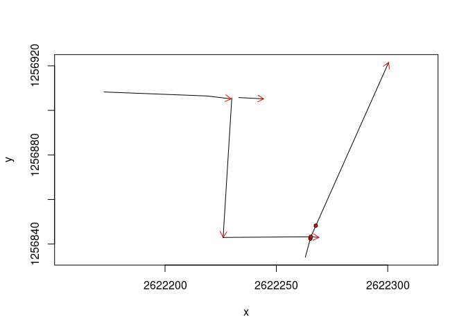 The red arrows indicate the direction of the survey, the red dots the
fiducial markers and the circles the GPR profile intersections.
The red arrows indicate the direction of the survey, the red dots the
fiducial markers and the circles the GPR profile intersections.
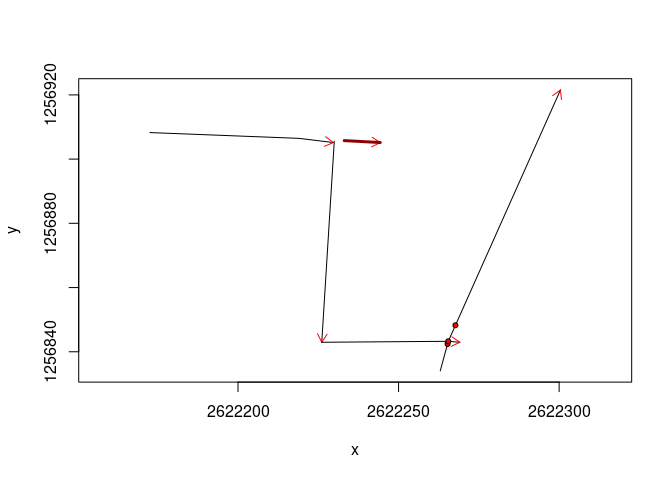
Highlight a GPR line:
plot(mySurvey)
lines(mySurvey[2], col = "darkred", lwd = 3)
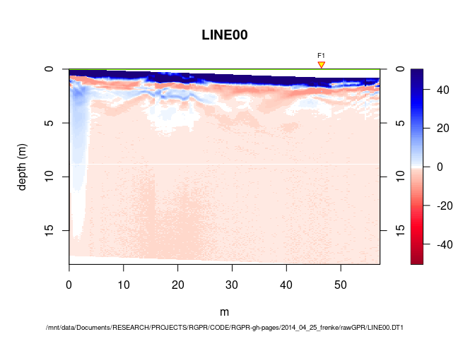
To plot the first GPR record, enter:
plot(mySurvey[[1]], addTopo=TRUE)
## time to depth conversion with constant velocity (0.1 m/ns)
To plot all the GPR records with the topographic information in 3D, enter:
plot3DRGL(mySurvey, addTopo = TRUE)
Enlarge the window, use the mouse to move the view and zoom in.
Once you found a satisfactory combination of processing steps, you can apply them all the GPR data. Here is an example
Create a sub-directory in the /processing directory (name it
mySurveyProc):
procDir <- file.path(getwd(), "processing/mySurveyProc")
dir.create(file.path(procDir), showWarnings = TRUE)
Now apply the processing step with a loop to all GPR data indexed by
mySurvey:
for(i in seq_along(mySurvey)){
  A <- mySurvey[[i]]            # get GPR-line no. i
  cat("processing of line", name(A),"      ")
  A <- dcshift(A, 1:100)          # DC-shift
  A <- gain(A, type = "power", alpha = 1, te = 200, tcst = 100)
  A <- fFilter(A, f= c(150, 200), type = "low", plotSpec = FALSE)
  A <- gain(A, type = "exp", alpha = 0.1, t0 = 50, te = 180)
  A <- dewow(A, type = "runmed", w = 50)              # dewow
  A <- filter2D(A, type = "median3x3")
  # export PDF
 exportPDF(A, clip = 30, fPath = file.path(procDir, name(A)), addTopo = TRUE,
          lwd = 0.5, ws = 1.5)
  # save the processed GPR-line into ".rds" format
  writeGPR(A, fPath = file.path(procDir, name(A)),
          type = "rds", overwrite = TRUE)
  cat("!\n")
}
Next time you can directly load the processed files as follows:
# select all the GPR files except CMP.DT1
procLINES <- file.path(procDir, paste0("LINE", sprintf("%02d", 0:4), ".rds"))
procSurvey <- GPRsurvey(procLINES)
and check the results:
plot(procSurvey[[1]], addTopo=TRUE)
plot3DRGL(procSurvey, addTopo = TRUE)
Create a list of lists defining the processing steps. The name of each
sublist (e.g., agc) correspond to the name of the processing function,
each sublist corresponds to the argument = values as defined by the
corresponding processing function. For example
prc <- list("gain"    = list(type = "agc", w = 10),
            "dewow"   = list(type = "Gaussian", w = 15),
            "fFilter" = list(f = c(10, 40, 150, 200), type = "bandpass",
                             plotSpec = FALSE))
Then, apply all the processing steps with the function papply() to the
GPRsurvey object mySurvey
mySurveyProc <- RGPR::papply(mySurvey, prc)
What do papply() do? It applies the processing steps as in the
for-loop in the previous section and stores locally the processed GPR
data on your local computer (temp files). That means that if you want to
use the processed GPR data in another R session, you still need to save
them manually, for example with the function writeGPR():
writeGPR(mySurveyProc, fPath = procDir, type = "rds")