Time/depth slice interpolation

Note:

This R-package is still in development, and therefore some of the functions may change in a near future.
If you have any questions, comments or suggestions, feel free to contact me (in english, french or german): emanuel.huber@pm.me.

Objectives of this tutorial
Preliminary
- Install/load the necessary packages
- Set the working directory
Read all the GPR data in a object of the class GPRsurvey
- Set the filepaths
- Create an object of the class GPRsurvey
Add coordinates
- Reverse GPR line direction (if necessary)
- Set grid coordinaes
Basic processing
Time/depth slice interpolation
Export slices as raster

Objectives of this tutorial

Learn how to assign coordinates to GPR data from a grid survey setup.
Learn how to interpolate time/depth slices.

However, this tutorial will not explain you the math/algorithms behind the different processing methods.

Preliminary

Download the repository GPRdata containing the data we will use along this tutorial
Unzip the data

We will work with the data contained in the directory /exampleDataCube/Grid-dir1-Rawdata/.

Install/load the necessary packages

if(!require("devtools")) install.packages("devtools")
devtools::install_github("emanuelhuber/RGPR")
library(RGPR)   # load RGPR in the current R session

[optionally] If RGPR is not installed, follow the instructions of the tutorial “Getting started” to install it.

Set the working directory

The working directory must be correctly set to use relative filepaths. The working directory can be set either in your R-software or in R directly with (of course you need to adapt the filepath shown below to your system):

DIR <- file.path("your_dir_path/GPRdata-master/exampleDataCube")
setwd(DIR)    # set the working directory
getwd()         # Return the current working directory (just to check)

Read all the GPR data in a object of the class `GPRsurvey`

An object of the class GPRsurvey is like an index that contains some of the meta-data of several GPR data recorded during one survey. With the class GPRsurvey you have an overview of all your data, you can compute the positions of the profile intersections, plot a top view of the survey and plot the data in 3D with open-GL (implemented in the R-package RGL).

Set the filepaths

Read all the GPR records (“.DZT”) located in the directory /exampleDataCube/Grid-dir1-Rawdata/

LINES <- file.path( paste0("FILE____", sprintf("%03d", 1:46), ".DZT"))

sprintf format the integer values ranging from 1 to 46 such that they match the file names (e.g., 1 becomes "001", 2 becomes "002", …, 46 becomes "046"). The 0 in "%03d" means pad with zeros to the field, 3 means that the field length is 3, d that the values are integer.

Create an object of the class `GPRsurvey`

SU <- GPRsurvey(LINES, verbose = FALSE)

Have a look at the newly created object:

SU

## *** Class GPRsurvey ***
## Unique directory:.
## - - - - - - - - - - - - - - -
##           name length units       date freq coord int        filename
## 1  FILE____001    9.0     m 2013-10-29  400    NO  NO FILE____001.DZT
## 2  FILE____002    9.0     m 2013-10-29  400    NO  NO FILE____002.DZT
## 3  FILE____003    9.0     m 2013-10-29  400    NO  NO FILE____003.DZT
## 4  FILE____004    9.0     m 2013-10-29  400    NO  NO FILE____004.DZT
## 5  FILE____005    9.0     m 2013-10-29  400    NO  NO FILE____005.DZT
## 6  FILE____006    9.0     m 2013-10-29  400    NO  NO FILE____006.DZT
## 7  FILE____007    9.0     m 2013-10-29  400    NO  NO FILE____007.DZT
## 8  FILE____008    9.0     m 2013-10-29  400    NO  NO FILE____008.DZT
## 9  FILE____009    9.0     m 2013-10-29  400    NO  NO FILE____009.DZT
## 10 FILE____010    9.0     m 2013-10-29  400    NO  NO FILE____010.DZT
## 11 FILE____011    9.0     m 2013-10-29  400    NO  NO FILE____011.DZT
## 12 FILE____012    9.0     m 2013-10-29  400    NO  NO FILE____012.DZT
## 13 FILE____013    9.0     m 2013-10-29  400    NO  NO FILE____013.DZT
## 14 FILE____014    9.0     m 2013-10-29  400    NO  NO FILE____014.DZT
## 15 FILE____015    9.0     m 2013-10-29  400    NO  NO FILE____015.DZT
## 16 FILE____016    9.0     m 2013-10-29  400    NO  NO FILE____016.DZT
## 17 FILE____017    9.0     m 2013-10-29  400    NO  NO FILE____017.DZT
## 18 FILE____018    9.0     m 2013-10-29  400    NO  NO FILE____018.DZT
## 19 FILE____019    9.0     m 2013-10-29  400    NO  NO FILE____019.DZT
## 20 FILE____020    9.0     m 2013-10-29  400    NO  NO FILE____020.DZT
## 21 FILE____021    9.0     m 2013-10-29  400    NO  NO FILE____021.DZT
## 22 FILE____022    9.0     m 2013-10-29  400    NO  NO FILE____022.DZT
## 23 FILE____023    9.0     m 2013-10-29  400    NO  NO FILE____023.DZT
## 24 FILE____024    9.0     m 2013-10-29  400    NO  NO FILE____024.DZT
## 25 FILE____025    9.0     m 2013-10-29  400    NO  NO FILE____025.DZT
## 26 FILE____026    9.0     m 2013-10-29  400    NO  NO FILE____026.DZT
## 27 FILE____027    9.0     m 2013-10-29  400    NO  NO FILE____027.DZT
## 28 FILE____028    9.0     m 2013-10-29  400    NO  NO FILE____028.DZT
## 29 FILE____029    9.0     m 2013-10-29  400    NO  NO FILE____029.DZT
## 30 FILE____030    9.0     m 2013-10-29  400    NO  NO FILE____030.DZT
## 31 FILE____031    9.0     m 2013-10-29  400    NO  NO FILE____031.DZT
## 32 FILE____032    9.0     m 2013-10-29  400    NO  NO FILE____032.DZT
## 33 FILE____033    9.0     m 2013-10-29  400    NO  NO FILE____033.DZT
## 34 FILE____034    9.0     m 2013-10-29  400    NO  NO FILE____034.DZT
## 35 FILE____035    9.0     m 2013-10-29  400    NO  NO FILE____035.DZT
## 36 FILE____036    9.0     m 2013-10-29  400    NO  NO FILE____036.DZT
## 37 FILE____037    9.0     m 2013-10-29  400    NO  NO FILE____037.DZT
## 38 FILE____038    9.0     m 2013-10-29  400    NO  NO FILE____038.DZT
## 39 FILE____039    9.0     m 2013-10-29  400    NO  NO FILE____039.DZT
## 40 FILE____040    9.0     m 2013-10-29  400    NO  NO FILE____040.DZT
## 41 FILE____041    9.0     m 2013-10-29  400    NO  NO FILE____041.DZT
## 42 FILE____042    9.0     m 2013-10-29  400    NO  NO FILE____042.DZT
## 43 FILE____043    9.0     m 2013-10-29  400    NO  NO FILE____043.DZT
## 44 FILE____044    9.0     m 2013-10-29  400    NO  NO FILE____044.DZT
## 45 FILE____045    9.0     m 2013-10-29  400    NO  NO FILE____045.DZT
## 46 FILE____046    9.0     m 2013-10-29  400    NO  NO FILE____046.DZT
## ****************

You can see that no coordinates (x,y,z) are associated with the GPR data. Therefore, if you try to plot the survey you will get:

plot(SU, asp = 1) # throw an error

Add coordinates

The data come without coordinates. To add coordinate to GPR data, check the tutorial Adding coordinates to GPR data. Note that RPGR automatically reads GPS files associated with the GPR data and interpolate the trace positions.

Here, we assume that the data were collected on a grid: all the GPR data are parallel, oriented in the same direction and spaced by 0.20 m. For grid settings, a new approach is here introduced (here only with data recorded along the y-direction, but it works also for data recorded along the x-direction and along both direction). If your data already have coordinates, skip the section below.

Reverse GPR line direction (if necessary)

For this approach, all the data must be oriented in the same direction (the x-lines must have the same direction, the y-lines must have the same direction). If this is not the case for your data, you can use the function reverse() to reverse the GPR line. You can specify which lines must be reversed:

SU <- reverse(SU, id = seq(from = 2, to = 11, by = 2))

or if your data were collected in zig-zag (two adjacent GPR lines have opposite direction), you can use the argument "zigzag":

#all the even GPR lines are reversed
SU <- reverse(SU, id = "zigzag")

Set grid coordinaes

Specifications

To set the grid coordinates, use the function setGridCoord() and assign the grid specifications in the form of a list. This list takes for arguments (see also:

xlines: integer values corresponding to the x-lines in the GPRsurvey object (if there are no x-lines, no need to specify xlines).
xpos: the position of the x-lines along the x-axis, same length as xlines (if there are no x-lines, no need to specify xpos).
xstart[optional]: shift to apply along the y-position, useful if the lines do not start at the same position; same length as xlines (if there are no x-lines, no need to specify xstart).
xlength[optional]: the length of the lines. Note that normally RGPR reads the line length from the data (if there are no x-lines, no need to specify xlength).
ylines: integer values corresponding to the x-lines in the GPRsurvey object (if there are no y-lines, no need to specify ylines).
ypos: the position of the x-lines along the x-axis, same length as ylines (if there are no y-lines, no need to specify ypos).
ystart[optional]: shift to apply along the x-position, useful if the lines do not start at the same position; same length as ylines (if there are no y-lines, no need to specify ystart).
ylength[optional]: the length of the lines. Note that normally RGPR reads the line length from the data (if there are no y-lines, no need to specify ylength).

Note that:

the length of xlines, xpos, xstart and xlength must be equal (except if you omit xstart and/or xlength)
the length of ylines, ypos, ystart and ylength must be equal (except if you omit ystart and/or ylength)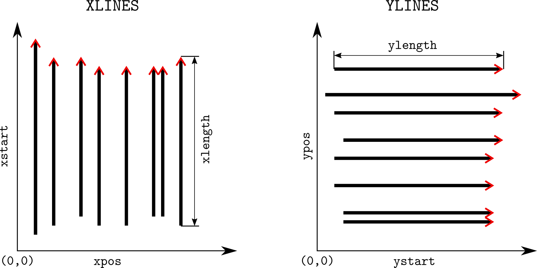

Visualisation of the grid specification
arguments

Example 1

Imagine your data were collected as follows:

40 x-lines with line spacing = 2 m; the 3rd and 5th lines start 1 m after the other lines.
6 y-lines at positions 0 m, 1 m, 2 m, 4 m, 6 m, and 7.6 m; the 1st line start 2 m before the other lines.

SU_img <- SU
xstart <- rep(0, 40)
xstart[c(3, 5)] <- 1
setGridCoord(SU_img) <- list(xlines = 1:40,
                         xpos   = seq(0, by = 2, length.out = 40),
                         xstart = xstart,
                         ylines = 40 + (1:6),
                         ypos   = c(0, 1, 2, 4, 6, 7.6),
                         ystart = c(-2, 0, 0, 0, 0, 0))
plot(SU_img, asp = TRUE, parFid = NULL)

Example 2

Imagine your data were collected on a 19 m x 25m grid:

20 x-lines and 26 y-lines
1 m line spacing (in both x- and y-directions)
x-length is 25 m and y-length is 19 m (assuming that RGPR did not read the correct GPR line length)
all the lines start either at x = 0 m or at y = 0 m

SU_img <- SU
setGridCoord(SU_img) <- list(xlines = 1:20,
                         xpos = seq(0, by = 1, length.out = 20),
                         xstart = rep(0, 20),  # could be omitted
                         xlength = rep(25, 20),
                         ylines =  21:46,
                         ypos = seq(0, by = 1, length.out = 26),
                         ystart = rep(0, 26),  # could be omitted
                         ylength = rep(19, 26))

plot(SU_img, asp = TRUE, parFid = NULL)

Case study

In our case we have only x-lines, so we don’t specify ylines, ypos, and ystart. The 5th, 8th, 22th lines starts 1 m after the others; the 1st, 28th, 33rd, 38th, and 44th lines start 0.4 m after the others:

# define xstart
xstart <- rep(0, length(SU))
xstart[c(5, 8, 22)] <- 1
xstart[c(1, 28, 33, 38, 44)] <- 0.4
setGridCoord(SU) <- list(xlines = seq_along(SU),
                         xpos   = seq(0, by = 0.2,
                                      length.out = length(SU)),
                         xstart = xstart)

Now you can plot your survey data (because you have coordinates)

plot(SU, asp = TRUE, parFid = NULL)

We set parFid = NULL because we do not want to plot all the fiducial markers

Basic processing

Plot a single GPR data with

plot(SU[[1]])

## Antenna separation set to 0 m. Set it with 'antsep(x) <-... '

You see that some processing is needed.

We apply some basic processing steps sequentially (estimate time-zero and shift all the traces to time-zero, dewow, AGC-gain). Maybe you want to horizontally smooth the data (un-comment the line starting traceStat) or to interpolate the signal envelope (un-comment the line starting envelope). For more info on GPR data processing check the tutorial Basic GPR data processing

SU <- papply(SU,
             prc = list(estimateTime0 = list(method = "coppens", w = 2),
                        # "NULL" because we take the default
                        time0Cor = NULL,
                        dewow = list(w = 3),
                        gain = list(type = "agc", w = 1.2) #,
                        # traceStat = list(w = 20, FUN = mean),
                        # envelope = NULL)
))

Does it look better now?

plot(SU[[1]])

Time/depth slice interpolation

Now that the data are well prepared, the interpolation is a simple task. We define the grid resolution in all three direction: dx = 0.05 m, dy = 0.05 m, dz = 0.05 ns as well as an additional parameter h (>0) that controls the smoothness of the interpolation (the interpolation used is the Multilevel B-spline Approximation as implemented in the function mba.surf() of the package MBA).

SXY <- interpSlices(SU, dx = 0.05, dy = 0.05, dz = 0.05, h = 6)
SXY

## *** Class GPRcube ***
## dim:    199 x 219 x 901
## res:    0.05 m x 0.05 m x 0.05 ns
## extent: 9.9 m x 10.9 m x 45 ns
## crs:
## *********************

How to manipulate a `GPRcube` object

SXY can be manipulated like an array with x, y and z dimensions.

Plot an horizontal slice of the data cube:

plot(SXY[,,10])

Plot a vertical slice along x-direction

plot(SXY[,10,])

Plot a vertical slice along y-direction

plot(SXY[10,,])

Color palette

You can define the same color range for each plot:

# color range (over all possible slice values)
clim <- range(SXY, na.rm = TRUE)
plot(SXY[,,50], clim = clim)

You can change the color palette? displayPalGPR() shows all the palette available in RGPR

displayPalGPR()

Try these two palettes: "sunny" and "slice":

plot(SXY[,,50], clim = clim, col = palGPR("sunny"), asp = 1)

plot(SXY[,,50], clim = clim, col = palGPR("slice"), asp = 1)

Specify the interpolation extend

By defaut the slices are interpolated whithin the convex hull of the GPR lines that is extended by 5 percents.

It is possible to specify the type of interpolation extend with the argument extend that can take the following values:

chull: the convex-hull
bbox: the axis-aligned bounding box
obbox: the oriented bounding box
buffer: an area around the GPR lines (like a buffer). In this case a buffer value> 0 must be defined.

Below are some examples (the case extend = "obbox" makes here no sense because the oriented bounding-box is the same as the axis-aligned bounding box).

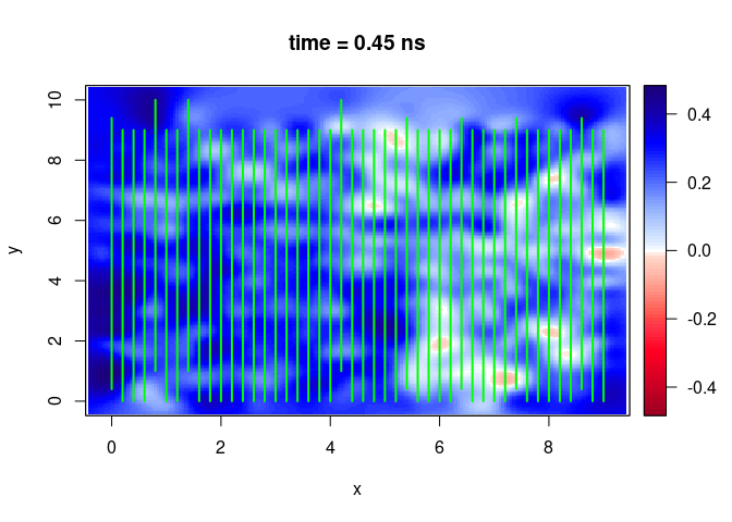
SXY <- interpSlices(SU, dx = 0.05, dy = 0.05, dz = 0.05, h = 6, extend = "chull", buffer = 0)
plot(SXY[,,10])
lines(SU, col = "green", lwd = 2)

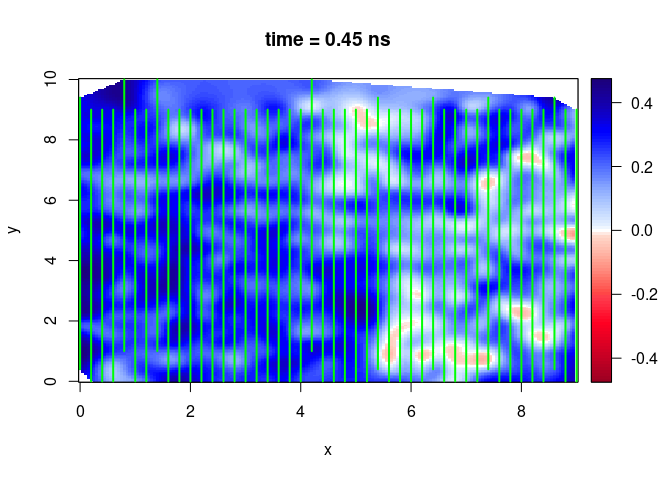
SXY <- interpSlices(SU, dx = 0.05, dy = 0.05, dz = 0.05, h = 6, extend = "chull", buffer = 2)
plot(SXY[,,10])
lines(SU, col = "green", lwd = 2)

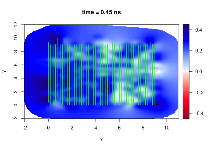
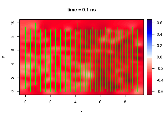
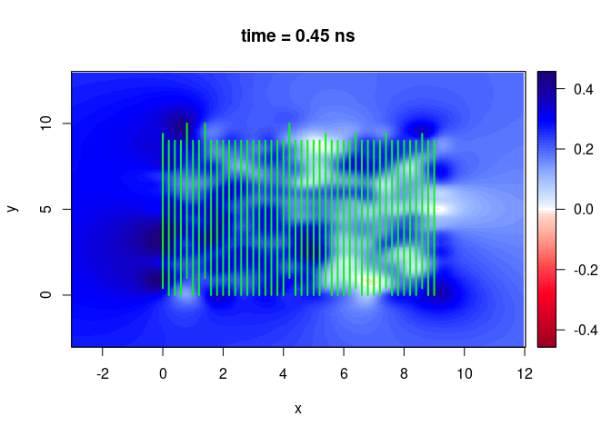
SXY <- interpSlices(SU, dx = 0.05, dy = 0.05, dz = 0.05, h = 6, extend = "bbox")
plot(SXY[,,3])
lines(SU, col = "green", lwd = 2)

SXY <- interpSlices(SU, dx = 0.05, dy = 0.05, dz = 0.05, h = 6, extend = "bbox", buffer = 3)
plot(SXY[,,10])
lines(SU, col = "green", lwd = 2)

SXY <- interpSlices(SU, dx = 0.05, dy = 0.05, dz = 0.05, h = 6, extend = "obbox")
plot(SXY[,,10])
lines(SU, col = "green", lwd = 2)

SXY <- interpSlices(SU, dx = 0.05, dy = 0.05, dz = 0.05, h = 6, extend = "obbox", buffer = 3)
plot(SXY[,,10])
lines(SU, col = "green", lwd = 2)

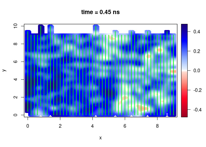
SXY <- interpSlices(SU, dx = 0.05, dy = 0.05, dz = 0.05, h = 6, extend = "buffer", buffer = 0.2)
plot(SXY[,,10])
lines(SU, col = "green", lwd = 2)

Export slices as raster

You first need to convert the slice you want to export into a raster object in R (defined in the raster package):

r <- as.raster(SXY[,,10])

## The legacy packages maptools, rgdal, and rgeos, underpinning the sp package,
## which was just loaded, will retire in October 2023.
## Please refer to R-spatial evolution reports for details, especially
## https://r-spatial.org/r/2023/05/15/evolution4.html.
## It may be desirable to make the sf package available;
## package maintainers should consider adding sf to Suggests:.
## The sp package is now running under evolution status 2
##      (status 2 uses the sf package in place of rgdal)

Then, use the writeRaster() function of the raster package to export the slice in the raster format you like (check the help on this function, ?raster::writeRaster):

raster::writeRaster(r, filename = "slice10.tif")

You may also want to export the coordinates as shapefiles or geodata, as lines

exportCoord(SU, type = c("SpatialLines"), fPath = "myshapefile.shp",
            driver = "ESRI Shapefile")

… or as points

exportCoord(SU, type = c("SpatialPoints"), fPath = "myshapefile.shp",
            driver = "ESRI Shapefile")

Adapt the driver and the filename extension to your need (for that, check the help on the rgdal::writeOGR() function).

Time/depth slice interpolation

Table of Contents

Objectives of this tutorial

Preliminary

Install/load the necessary packages

Set the working directory

Read all the GPR data in a object of the class GPRsurvey

Set the filepaths

Create an object of the class GPRsurvey

Add coordinates

Reverse GPR line direction (if necessary)

Set grid coordinaes

Specifications

Example 1

Example 2

Case study

Basic processing

Time/depth slice interpolation

How to manipulate a GPRcube object

Color palette

Specify the interpolation extend

Export slices as raster

Read all the GPR data in a object of the class `GPRsurvey`

Create an object of the class `GPRsurvey`

How to manipulate a `GPRcube` object