GPR data deconvolution

Note:

• This R-package is still in development, and therefore some of the functions may change in a near future.
• If you have any questions, comments or suggestions, feel free to contact me (in english, french or german): emanuel.huber@pm.me.

Table of Contents

• Objectives of this tutorial
• Preliminary
  • Install/load RGPR
  • Read the data
• GPR data deconvolution
  • First wave break and time zero estimation
  • DC-shift
  • Time zero correction
  • Dewow
  • Frequency filter
  • Time gain
  • Mixed phase deconvolution
    • Minimum-phase deconvolution and phase rotation
    • Minimum-phase and mixed-phase wavelet
  • Frequency filter
  • Trace scaling
  • Comparison

Objectives of this tutorial

• Learn how to apply the deconvolution scheme of Schmelzbach and Huber (2015) to GPR data

Note that his tutorial will not explain you the math/algorithms behind the different processing methods.

We follow the approach proposed by Schmelzbach and Huber (2015), Efficient Deconvolution of Ground-Penetrating Radar Data, IEEE Transactions on Geosciences and Remote Sensing 53 (9), 5209-5217, doi:10.1109/TGRS.2015.2419235.

Download the pdf

Preliminary

• Read the tutorial Basic GPR data processing to learn more about the processing methods
• Download the data 2012_10_06_cornino.zip. The data can be also downloaded on Zenodo and can be cited as follow: Huber, Emanuel (2019), GPR data used to test the efficient deconvolution method of Schmelzbach and Huber (2015), doi:10.5281/zenodo.2586189.
• Unzip the data

Install/load RGPR

• Install/load RGPR

  # install "devtools" if not already done
  if(!require("devtools")) install.packages("devtools")
  devtools::install_github("emanuelhuber/RGPR")
  library(RGPR)       # load RGPR in the current R session
  

• Set the working directory:

  DIR <- "~/2012_10_06_cornino"  # adapt that to your directory structure
  setwd(DIR)    # set the working directory
  getwd()         # Return the current working directory (just to check)
  

Read the data

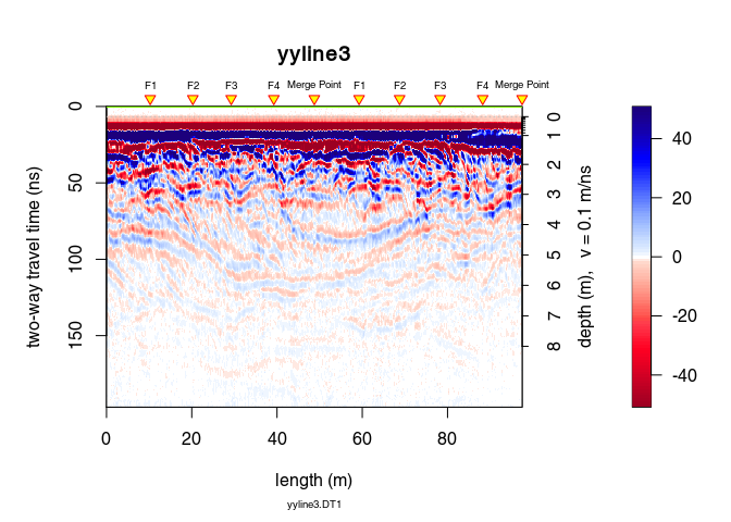
x <- readGPR(dsn = "yyline3.DT1")
x <- x[1:300, ]

GPR data deconvolution

First wave break and time zero estimation

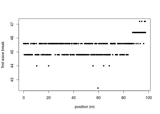
Quantify first wave break:

tfb <- firstBreak(x, w = 20, method = "coppens", thr = 0.05)
plot(pos(x), tfb, pch = 20, ylab = "first wave break",
     xlab = "position (m)")

Convert first wave break to time-zero and set time-zero

t0 <- firstBreakToTime0(tfb, x)
time0(x) <- mean(t0)     # set time0

DC-shift

x1 <- dcshift(x)

Time zero correction

To shift the traces to time-zero, use the function time0Cor (the method argument defines the type of interpolation method)

x2 <- time0Cor(x1, method = "pchip")

Dewow

Remove the low-frequency components (the so-called “wow”) of the GPR record:

x3 <- dewow(x2, type = "runmed", w = 50)     # dewowing:
plot(x3)                                     # plot the result

plot(x3 - x2)                           # plot the difference

Frequency filter

To remove low (dewow) and high (noise) frequency (large bandpass to minimise the introduction of artifact)

x4 <- fFilter(x3, f = c(5, 20, 300, 400), type = "bandpass",
                plotSpec = TRUE)

Time gain

Apply a power gain and a spherical gain to compensate for geometric wave spreading and attenuation (Kruse and Jol, 2003; Grimm et al., 2006).

# power gain (compensate geometric spreading)
x5 <- gain(x4, type ="power",  alpha = 1, t0 = 0, te = 200)
# exponential gain (compensate for attenuation)
x6 <- gain(x5, type ="exp",  alpha = 0.023, t0 = 30, te = 180)

trPlot(traceStat(envelope(x4)), col = "red", main="")
trPlot(traceStat(envelope(x5)), col = "blue", add=TRUE)
trPlot(traceStat(envelope(x6)), col = "green", add=TRUE)
legend("topright",legend=c("before","power gain", "exponential gain"),
       lwd=c(1,1,1), col=c("red","blue","green"))

Mixed phase deconvolution

Select the time window on which the deconvolution will be applied:

tWin <- c(32, 112)  # ns
W <- which(depth(x6) > tWin[1] & depth(x6) < tWin[2])

plot(x6[W, ], main = "selected time window")

Minimum-phase deconvolution and phase rotation

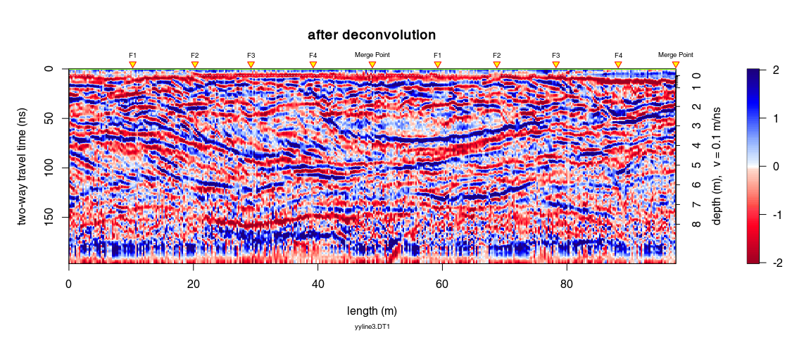
Apply the mixed-phase deconvolution: spiking deconvolution + phase rotation that maximise the kurtosis of the GPR data.

x_dec <- deconv(x6, method="mixed-phase", W = tWin, wtr = 5, nf = 35,
                mu = 0.00001)

Estimated phase rotation: 103.13°.

The function deconv() (when method = "mixed-phase") returns a list of following elements:

• fmin: estimated inverse minimum-phase wavelet
• wmin: estimated minimum-phase wavelet
• optRot: rotation of the minimum-phase wavelet that maximise the kurtosis
• wmix: estimated mixed-phase wavelet (the rotated minimum-phase wavelet)
• x: the deconvolued data

You can compare the results with the “minimum-phase deconvolution” also called “spiking deconvolution” by setting in deconv() method = "spiking" (in this case, deconv() returns only fmin, wmin and x).

Minimum-phase and mixed-phase wavelet

In black the estimated wavelets for each trace, in red the mean wavelet.

w_min <- x_dec$wmin
w_mix <- x_dec$wmix


par(mfrow=c(1,2))
plot(0,0,type="n",xlim=range(w_min$x), ylim = max(abs(w_mix$y))*c(-1,1),
      xaxs = "i", xlab = "time (ns)", ylab = "amplitude",
    main = "minimum-phase wavelet")
grid()
apply(w_min$y,2,lines, x = w_min$x, col=rgb(0.2,0.2,0.2,0.2))
lines(w_min$x, apply(w_min$y,1,mean), col="red", lwd=3)


plot(0,0,type="n",xlim=range(w_mix$x),ylim=max(abs(w_mix$y))*c(-1,1),
    xaxs = "i", xlab = "time (ns)", ylab = "amplitude",
    main = "mixed-phase wavelet")
grid()
apply(w_mix$y,2,lines, x = w_mix$x, col=rgb(0.2,0.2,0.2,0.2))
lines(w_mix$x, apply(w_mix$y,1,mean), col="red", lwd=3)

Frequency filter

To remove the high-frequency noise boosted by the deconvolution

x7 <- fFilter(x_dec$x, f = c(5, 20, 160, 210), type = "bandpass",
                    plot = TRUE)

Trace scaling

x8 <- traceScaling(x7, type="stat")

Comparison

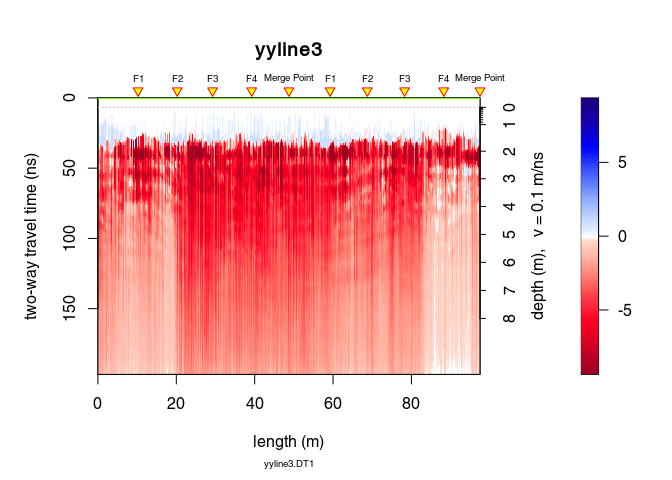
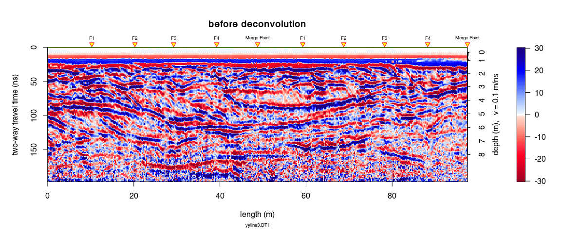
plot(x6, main = "before deconvolution", clip = 30)

plot(x8, main = "after deconvolution",  clip = 2)