Implementation

1. Cholesky decomposition

The Cholesky decomposition of a Hermitian positive-definite matrix $\mathbf{A}$ is

with $L$ a lower triangular matrix .

2. Solving and computing with Cholesky decomposition

2.a. Solve $A x = b$ for $x$

Solve $A x = b$ for $x$ knowing that $A = LL^T$, with $L$ a lower triangular matrix.

We write $\alpha = L^T x$.

1. Solve $L \alpha = b$ for $\alpha$ by forward substitution.
2. Solve $L^T x = \alpha$ for $x$ by backward substitution.

2.b. Compute $H^T A^{-1} H$

Compute $H^T A^{-1} H$ knowing that $A = LL^T$, with $L$ a lower triangular matrix.

with $v = L^{-1}H$

1. Solve $Lv = H$ for $v$ by forward substitution.
2. Compute the crossproduct $v^Tv$.

2.c. Compute $K_\star^T K^{-1} y$

Compute $K_\star^T K^{-1} y$ knowing that $K_\star$ and $K$ are positive-definite, and $K = LL^T$ with $L$ a lower triangular matrix.

with $b = L^{-1}K_\star$ and $a = L^{-1}y$

1. Solve $Lb = K_\star$ for $b$ by forward substitution.
2. Solve $La = y$ for $a$ by forward substitution.
3. Compute the cross-product $b^Ta$!

3. Predictions and log marginal likelihood for Gaussian process regression

See book of Rasmussen and Williams (2006), chap. 2, page 19.

Predictive mean: $\bar{f_\star} = K_\star^T (K + \sigma^2 I)^{-1}y$

Predictive variance: $Var(f_\star) = K_{\star\star}^T - K_\star^T (K + \sigma^2 I)^{-1}K_\star$

Algorithm of Rasmussen and Williams (2006):

1. $L \leftarrow \text{cholesky}(K + \sigma^2 I)$
2. $\alpha \leftarrow L^T(L\y)$
3. $\bar{f_\star} \leftarrow K_\star^T \alpha$
4. $v \leftarrow L\K_\star$
5. $Var(f_\star) \leftarrow K_{\star\star} - v^T v$
6. $\log(p(y\mid X)) \leftarrow -\frac{1}{2} y^T \alpha - \sum_i \log L_{ii} - \frac{n}{2}\log 2\pi$

Algorithm of GauProMod, file GPpred.cpp (note that here we write $K$ for $(K + \sigma^2 I)$):

1. Compute $L$ with the cholesky decomposition, i.e.,

    L = K.llt().matrixL());
   

2. We compute $b^T = (L^{-1}K_\star)^T$ by solving $L^Tb^T = K_\star^T$ for $b^T$ (see Section 2.c.1)

    bt = (L.triangularView<Lower>().solve(Kstar)).adjoint();
   

3. We compute $a = L^{-1}y$ by solving $La = y$ for $a$ (see Section 2.c.2)

    a = L.triangularView<Lower>().solve(y);
   

4. We compute the mean of the Gaussian process: $\bar{f_\star} = b^Ta = K_\star^T K^{-1}y$

    M = bt * a;
   

5. We compute $K_\star^T (K + \sigma^2 I)^{-1}K_\star = v^T v$ (see Section 2.b)

    btb = MatrixXd(kk,kk).setZero().selfadjointView<Lower>().rankUpdate(bt);
   

6. We compute the covariance of the Gaussian process: $Var(f_\star) = K_{\star\star}^T - K_\star^T (K + \sigma^2 I)^{-1}K_\star$

    C = Kstarstar - vtv;
   

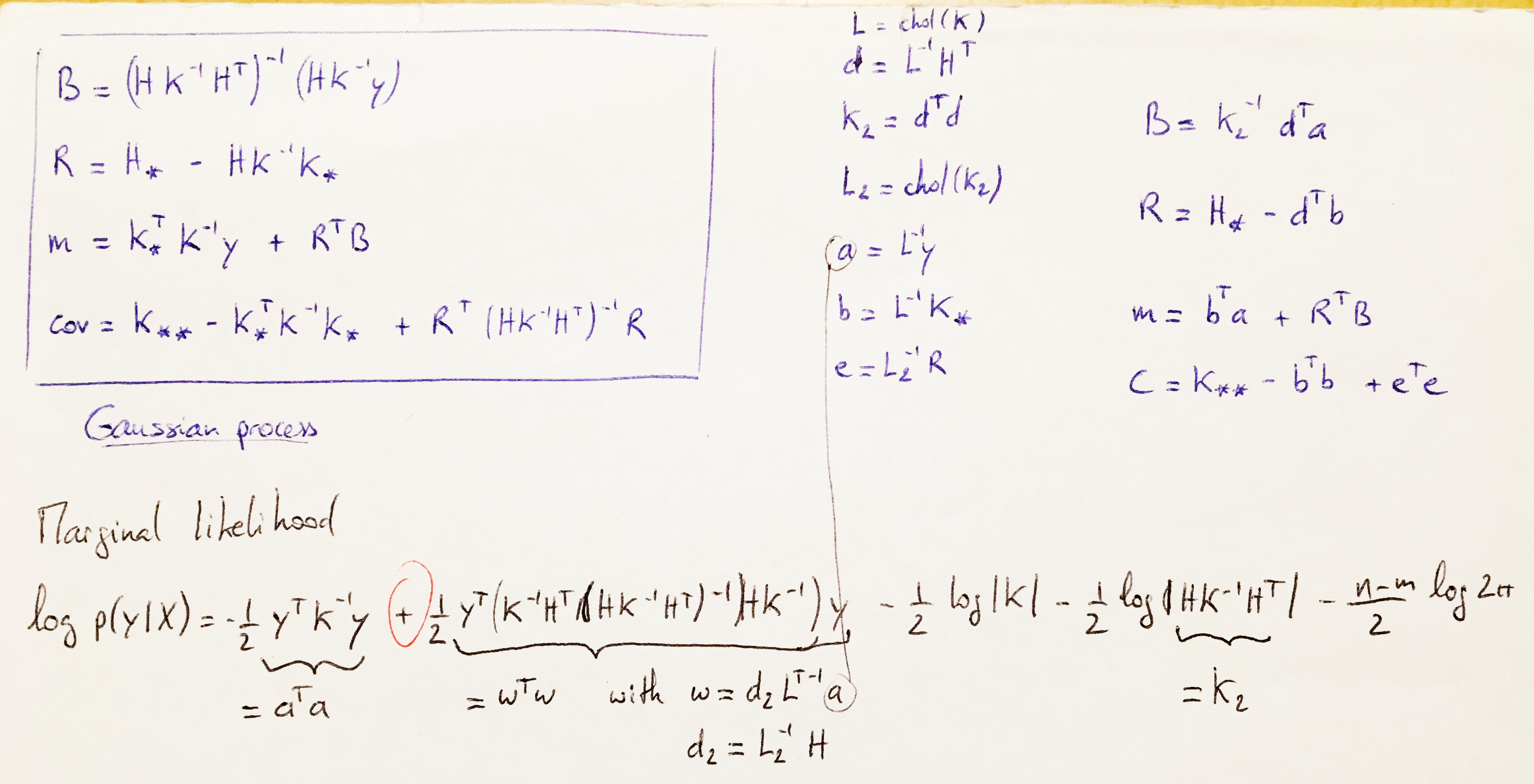
4. Predictions and log marginal likelihood for Gaussian process regression with explicit basis functions

See book of Rasmussen and Williams (2006), chap. 2.7, page 27-29.

Algorithm of GauProMod, file GPpredmean.cpp:

See my notes…

5. Log determinant of positive definite matrices

Knowing that:

1. Cholesky decomposition of positive definite matrix $\mathbf{A}$

   $$\mathbf{A} = \mathbf{L}\mathbf{L}^T$$

2. determinant of a positive definite matrix $\mathbf{A}$:

   $$\begin{aligned} \det(\mathbf{A}) &= \det(\mathbf{L}\mathbf{L}^T)\\ &= \det(\mathbf{L})\det(\mathbf{L}^T)\\ &= \det(\mathbf{L})^2 \end{aligned}$$

3. log rule

   $$\log \prod_i x_i = \sum_i \log x_i$$

4. determinant of a lower triangular matrix

   $$\det(\mathbf{L}) = \prod_i L_{ii}$$

the log determinant of positive definite matrices is:

Thus to calculate the log determinant of a symmetric positive definite matrix in R:

L <- chol(A)
logdetA <- 2*sum(log(diag(L)))

6. Determinant od the exponential of a matrix $\mathbf{B}$

See the proof here