Tutorial
How to install/load
if(!require("devtools")) install.packages("devtools")
devtools::install_github("emanuelhuber/GauProMod")
Short tutorial
Load libraries
library(GauProMod)
library(plot3D)
library(RColorBrewer)
1D Gaussian Process Modelling
Observations and target
The observations are defined by a list with x the positions of the observations and y the observed values. The targets are the positions x where to simulate the Gaussian Process.
#observations
obs <- list(x=c(-4, -3, -1, 0, 4),
            y=c(-2,  0,  1, 2, 0))
# targets
targ <- list("x"=seq(-10,10,len=200))
Covariance function, mean function and likelihood
To build the covariance functions, the following kernels are available
# linear kernel
covModel <- list(kernel="linear",
                 b = 1,         # slope
                 h = 1.5,       # std. deviation
                 c = 0)         # constant

# Matern kernel
covModel <- list(kernel="matern",
                 l = 1,       # correlation length
                 v = 2.5,     # smoothness
                 h = 2.45)    # std. deviation

# squared exponential kernel (Gaussian)
covModel <- list(kernel="gaussian",
                 l = 0.5,   # correlation length
                 h = 0.25)  # std. deviation
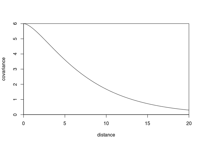
Covariance as a function of distance
covModel <- list(kernel="matern",
                 l = 5,     # correlation length
                 v = 1,     # smoothness
                 h = 2.45   # std. deviation
                )
r <- seq(0, 20, by = 0.1)
myCov <- covfx(r = r, covModel = covModel)
plot(r, myCov, type = "l", ylim = c(0, max(myCov)),
     ylab = "covariance", xlab = "distance", xaxs = "i", yaxs = "i")
The following mean function (or basis functions) are available (see Rasmussen and Williams (2006), Section 2.7):
# quadratic mean function
op <- 2
# linear mean function
op <- 1
# zero-mean function (no trend)
op <- 0
Because nothing is perfectly observed, it makes sense to account for uncertainty in the observation. Gaussian likelihood, defined by the standard deviation sigma (erreur uncertainty) is the only form of likelihood currently implemented in GauProMod. Sigma must be either a length-one vector or has exactly the same length as the observations values
# standard deviation measurement error
# Gaussian likelihood
sigma <- 0.2
# or
sigma <- abs(rnorm(length(obs$y)))
Conditional Gaussian Process modelling
GP <- gpCond(obs = obs, targ = targ, covModels=list(pos=covModel),
               sigma = sigma, op = op)
names(GP)
# GP$mean   = mean value at location xstar
# GP$cov    = covariance matrix of the conditioned GP
# GP$logLik = log-likelihood of the conditioned GP
# GP$xstar  = x-coordinates at which the GP is simulated
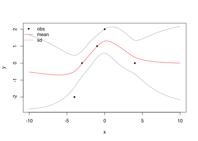
Plot the mean function plus/minus the standard deviation
#--- plot mean +/- sd
xp <-(GP$mean + sqrt(diag(GP$cov)))  # mean + sd
xm <-(GP$mean - sqrt(diag(GP$cov)))  # mean - sd

# initialise the plot
plot(cbind(obs$x, obs$y), type="p", xlab="x", ylab="y",
     xlim = range(c(obs$x, targ$x)), ylim = range(c(xp, xm, obs$y)),
     pch = 20, col = "black")
lines(GP$xstar, GP$mean,col="red")  # mean
lines(GP$xstar, xm,lty=3)            # + sd
lines(GP$xstar, xp,lty=3)            # - sd
legend("topleft", legend = c("obs", "mean", "sd"), lty = c(NA, 1, 3),
       pch = c(20, NA, NA), col=c("black", "red", "black"), bty="n")
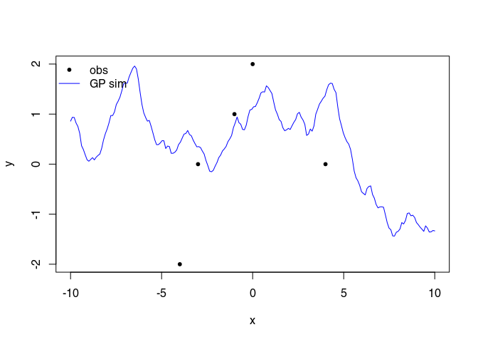
Random conditional simulation
# cholesky factorisation
L <- cholfac(GP$cov)
# random simulation
ystar <- gpSim(GP , L = L)
You can also directly use ystar <- gpSim(GP) without the argument L (the Cholesky factor) but each time you will call gpSim(GP), gpSim will compute again internally the Cholesky factor. So, if you plan to run many unconditional simulations, it is faster to first compute the Cholesky factor and then run several time gpSim with the argument L.
Plot the random simulation:
plot(rbind(cbind(obs$x, obs$y), ystar), type="n", xlab="x", ylab="y")
lines(ystar, col = "blue")
points(cbind(obs$x, obs$y), col = "black", pch = 20)
legend("topleft", legend = c("obs", "GP sim"), lty = c(NA, 1),
       pch = c(20, NA), col=c("black", "blue"), bty="n")
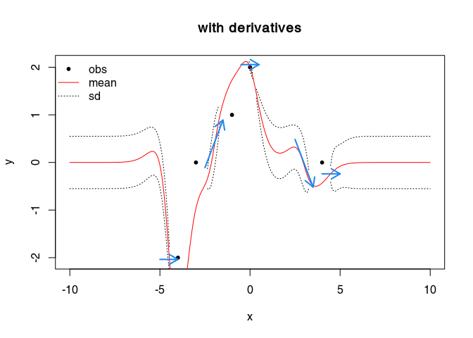
Conditional Gaussian Process modelling with derivatives
We define a new object bc (a list) defining the derivatives, with elements:
xthe location of the derivativeythe value of the derivativesigmathe uncertainty (standard deviation) on the derivative value (y)
covModel <- list(kernel = "matern",
                 l = 0.25,
                 v = 3.5,
                 h = 0.55)

bc <- list(x = c(-4.5, -2, 0,  3, 4.5),
           y = c(   0,  1, 0, -1,   0),
           sigma = 0)

sigma <- 0.1

GP <- gpCond(obs = obs, targ = targ, covModels=list(pos=covModel),
               sigma = sigma, op = 0)
GP2 <- gpCond(obs = obs, targ = targ, covModels=list(pos=covModel),
               sigma = sigma, op = 0, bc = bc)


#--- plot mean +/- sd
xp <-(GP$mean + sqrt(diag(GP$cov)))  # mean + sd
xm <-(GP$mean - sqrt(diag(GP$cov)))  # mean - sd
xp2 <-(GP2$mean + sqrt(diag(GP2$cov)))  # mean + sd
## Warning in sqrt(diag(GP2$cov)): NaNs produced
xm2 <-(GP2$mean - sqrt(diag(GP2$cov))) # mean - sd
## Warning in sqrt(diag(GP2$cov)): NaNs produced
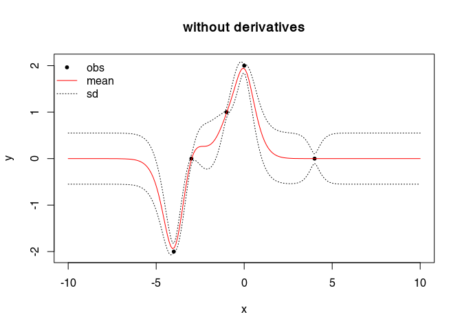
plot(cbind(obs$x, obs$y), type="p", xlab="x", ylab="y",
     xlim = range(c(obs$x, targ$x)), ylim = range(c(xp, xm, obs$y)),
     pch = 20, col = "black", main = "without derivatives")
lines(GP$xstar, GP$mean,col="red")  # mean
lines(GP$xstar, xm,lty=3)            # + sd
lines(GP$xstar, xp,lty=3)            # - sd
legend("topleft", legend = c("obs", "mean", "sd"), lty = c(NA, 1, 3),
       pch = c(20, NA, NA), col=c("black", "red", "black"), bty="n")
plot(cbind(obs$x, obs$y), type="p", xlab="x", ylab="y",
     xlim = range(c(obs$x, targ$x)), ylim = range(c(xp, xm, obs$y)),
     pch = 20, col = "black", main = "with derivatives")
lines(GP2$xstar, GP2$mean, col = "red")  # mean
lines(GP2$xstar, xm2,lty=3)            # + sd
lines(GP2$xstar, xp2,lty=3)            # - sd
legend("topleft", legend = c("obs", "mean", "sd"), lty = c(NA, 1, 3),
       pch = c(20, NA, NA), col=c("black", "red", "black"), bty="n")
y0 <- GP2$mean[sapply(bc$x, function(x, a) which.min(abs(x - a)), GP2$xstar)]
arrows(x0 = bc$x - 1/2, y0 = y0 - bc$y/2,
       x1 = bc$x + 1/2, y1 = y0 + bc$y/2,
       length = 0.15, col = "dodgerblue2", lwd = 2)
Gaussian Process Modelling with two dimensional “positions”
To understand everything, please read the previous section (“1D Gaussian Process Modelling”).
If you want to simulate a Gaussian process on a two-dimensional mesh, go to the section “2D Gaussian Process Modelling (simulation on a 2D mesh)”.
Observations and target
The observations are defined by a list with x the positions of the observations and y the observed values. Here, the element x of the observation list is a matrix corresponding to the coordinates of the observations points (East/North coordinates or x/y coordinates).
#observations
obs <- list(x = cbind(c(2.17, 7.92, 8.98, 7.77, 2.79, 5.36, 4.27, 3.07, 6.31),
                     c(1.33, 7.24, 4.26, 2.67, 6.17, 8.04, 3.18, 5.63, 8.33)),
            y = c(2.60, 1.48, 1.36, 8.61, 1.00, 1.58, 8.42, 8.39, 1.50))
The target is defined by a two-columns matrix corresponding to the coordinates of the target points.
# targets (=2D mesh)
targ <- list(x = cbind(c(2.17, 7.92, 8.98, 7.77, 2.79, 5.36, 4.27, 3.07, 6.31,
                       3.74, 5.93, 7.19, 6.61, 5.54, 2.27, 1.61, 4.02, 1.06),
                     c(1.33, 7.24, 4.26, 2.67, 6.17, 8.04, 3.18, 5.63, 8.33,
                       6.34, 3.68, 6.82, 1.79, 8.60, 7.73, 5.35, 2.45, 4.92))
                      )
Covariance function, mean function and likelihood
To build the covariance functions, the same kernels as in the previously defined are available:
# Matern kernel
covModel <- list(kernel="matern",
                 l = 5,     # correlation length
                 v = 1,     # smoothness
                 h = 2.45   # std. deviation
                )
Note that the 2D mean functions (or basis functions) are differently defined:
# 2D quadratic mean function
op <- 5
# zero-mean function (no trend)
op <- 0
# 2D linear mean function
op <- 2
Standard deviation (measurement error):
# Gaussian likelihood
sigma <- 0.2
Conditional Gaussian Process modelling
GP <- gpCond(obs = obs, targ = targ, covModels=list(pos=covModel),
               sigma = sigma, op = op)
names(GP)
# GP$mean   = mean value at location xstar
# GP$cov    = covariance matrix of the conditioned GP
# GP$logLik = log-likelihood of the conditioned GP
# GP$xstar  = x-coordinates at which the GP is simulated
# mean
Ymean <- GP$mean
# standard deviation
YSD <- sqrt(diag(GP$cov))
ysdplus <- Ymean - 1.95* YSD
ysdminus <- Ymean + 1.95* YSD
Results
Plot the mean and standard deviation functions
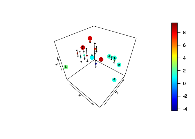
Three-dimensional plot
par(mfrow = c(1,1))
ylim <- range(Ymean, obs$y)
plot3D::scatter3D(x = targ$x[,1], y = targ$x[,2], z = Ymean, clim = ylim,
                  pch = 20)
plot3D::arrows3D(x0 = targ$x[,1], y0 = targ$x[,2], z0 = ysdminus,
                 x1 = targ$x[,1], y1 = targ$x[,2], z1 = ysdplus,
                 length=0.05, angle=90, code=3, add = TRUE, col = "black")
# large dots = observations
plot3D::scatter3D(x = obs$x[,1], y = obs$x[,2], z = obs$y, add = TRUE,
                  pch = 20, cex = 3, clim = ylim)
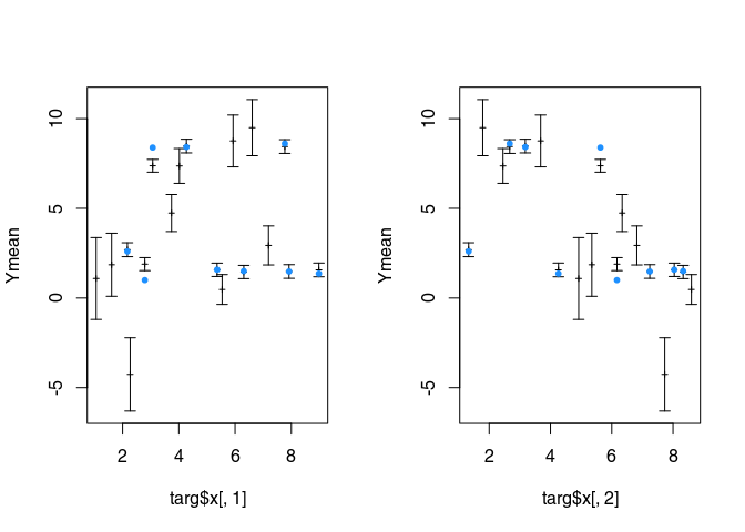
Pair of two-dimensional plots
par(mfrow = c(1, 2))
ylim <- range(ysdplus, ysdminus, obs$y)

plot(targ$x[,1], Ymean, type = "p", ylim = ylim, pch = 3, cex = 0.5)
arrows(targ$x[,1], ysdminus, targ$x[,1], ysdplus, length=0.05, angle=90, code=3)
points(obs$x[,1], obs$y, col = "dodgerblue", pch = 20)

plot(targ$x[,2], Ymean, type = "p", ylim = ylim, pch = 3, cex = 0.5)
arrows(targ$x[,2], ysdminus, targ$x[,2], ysdplus, length=0.05, angle=90, code=3)
points(obs$x[,2], obs$y, col = "dodgerblue", pch = 20)
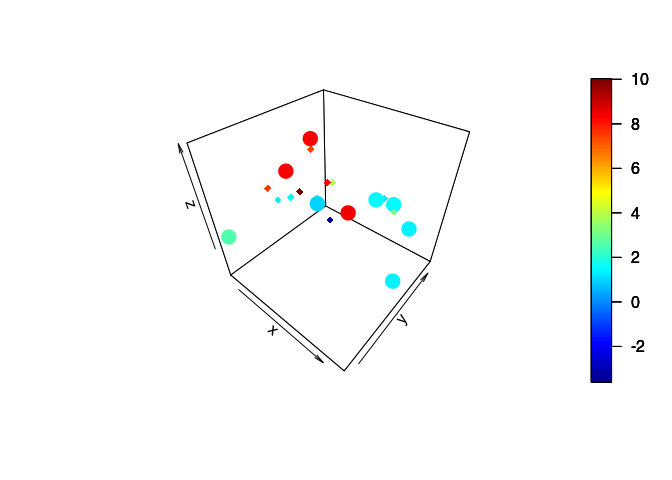
Random conditional simulation
L <- cholfac(GP$cov)
ystar <- gpSim(GP , L = L)

par(mfrow = c(1,1))
ylim <- range(ystar[,3], obs$y)
plot3D::scatter3D(x = targ$x[,1], y = targ$x[,2], z = ystar[,3], clim = ylim,
                  pch = 18)
# dots = observations
plot3D::scatter3D(x = obs$x[,1], y = obs$x[,2], z = obs$y, add = TRUE,
                  pch = 20, cex = 3, clim = ylim)
2D Gaussian Process Modelling (simulation on a 2D mesh)
To understand everything, please read the previous section (“1D Gaussian Process Modelling”).
Observations and target
The observations are defined by a list with x the positions of the observations and y the observed values. Here, the element x of the observation list is a matrix corresponding to the coordinates of the observations points (East/North coordinates or x/y coordinates).
#observations
obs <- list(x = cbind(c(2.17, 7.92, 8.98, 7.77, 2.79, 5.36, 4.27, 3.07, 6.31,
                       3.74, 5.93, 7.19, 6.61, 5.54, 2.27, 1.61, 4.02, 1.06),
                     c(1.33, 7.24, 4.26, 2.67, 6.17, 8.04, 3.18, 5.63, 8.33,
                       6.34, 3.68, 6.82, 1.79, 8.60, 7.73, 5.35, 2.45, 4.92)),
            y = c(2.60, 1.48, 1.36, 8.61, 1.00, 1.58, 8.42, 8.39, 1.50,
                  9.05, 1.14, 1.49, 9.19, 1.32, 1.03, 6.41, 6.16, 5.42))
The target is defined by a regular grid defined by two orthogonal vectors. The function vecGridreturns a two-columns matrix corresponding to the coordinates of each element of the grid.
# targets (=2D mesh)
vx <- seq(0, 10, by = 0.5)
vy <- seq(0, 10, by = 0.5)
targ <- list(x = vecGrid(vx, vy))
Covariance function, mean function and likelihood
To build the covariance functions, the same kernels as in the previously defined are available:
# linear kernel
covModel <- list(kernel="linear",
                 b = 1,         # slope
                 h = 0.5,       # std. deviation
                 c = 1)         # constant

# Matern kernel
covModel <- list(kernel="matern",
                 l = 1,       # correlation length
                 v = 2.5,     # smoothness
                 h = 2.45)    # std. deviation

# squared exponential kernel (Gaussian)
covModel <- list(kernel="gaussian",
                 l = 0.5,   # correlation length
                 h = 0.25)  # std. deviation
Note that the 2D mean functions (or basis functions) are differently defined:
# 2D quadratic mean function
op <- 5
# zero-mean function (no trend)
op <- 0
# 2D linear mean function
op <- 2
Standard deviation (measurement error):
# Gaussian likelihood
sigma <- 0.2
Conditional Gaussian Process modelling
GP <- gpCond(obs = obs, targ = targ, covModels=list(pos=covModel),
               sigma = sigma, op = op)
names(GP)
# GP$mean   = mean value at location xstar
# GP$cov    = covariance matrix of the conditioned GP
# GP$logLik = log-likelihood of the conditioned GP
# GP$xstar  = x-coordinates at which the GP is simulated
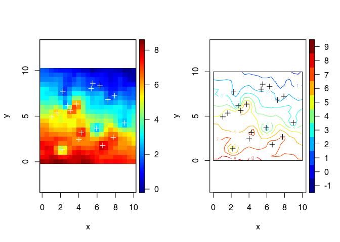
Plot the mean and standard deviation functions
# mean
Ymean <- matrix(GP$mean, nrow = length(vx), ncol = length(vy), byrow = TRUE)
# standard deviation
YSD <- matrix(sqrt(diag(GP$cov)), nrow = length(vx), ncol = length(vy),
              byrow = TRUE)

par(mfrow = c(2,2))
plot3D::image2D(x = vx, y = vy, z = Ymean, asp=1)
points(obs$x, col="white",pch=3)
title(main = "mean")

plot3D::contour2D(x = vx, y = vy, Ymean, asp=1)
points(obs$x, col="black",pch=3)
rect(vx[1], vy[1], vx[length(vx)], vy[length(vy)])
title(main = "mean")

plot3D::image2D(x = vx, y = vy, z = YSD, asp=1)
points(obs$x, col="white",pch=3)
title(main = "standard deviation")

plot3D::contour2D(x = vx, y = vy, YSD, asp=1)
points(obs$x, col="black",pch=3)
rect(vx[1], vy[1], vx[length(vx)], vy[length(vy)])
title(main = "standard deviation")

Random conditional simulation
L <- cholfac(GP$cov)
ystar <- gpSim(GP , L = L)

Ysim <- matrix(ystar[,3], nrow = length(vx), ncol = length(vy), byrow = TRUE)

par(mfrow=c(1,2))
plot3D::image2D(x = vx, y = vy, z = Ysim, asp=1)
points(obs$x, col="white",pch=3)


plot3D::contour2D(x = vx, y = vy, Ysim, asp=1)
points(obs$x, col="black",pch=3)
rect(vx[1], vy[1], vx[length(vx)], vy[length(vy)])
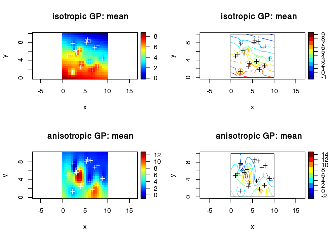
Anisotropy (scaling only along the coordinates axes)
covModelAni <- list(kernel="matern",
                 l = 1,       # correlation length
                 v = 2.5,     # smoothness
                 h = 2.45,
                 scale = c(1, 0.25))    # std. deviation
# 2D linear mean function
op <- 2

GP <- gpCond(obs = obs, targ = targ, covModels=list(pos=covModelAni),
               sigma = sigma, op = op)
names(GP)
# GP$mean   = mean value at location xstar
# GP$cov    = covariance matrix of the conditioned GP
# GP$logLik = log-likelihood of the conditioned GP
# GP$xstar  = x-coordinates at which the GP is simulated
Plot the mean and standard deviation functions
# mean
YmeanAni <- matrix(GP$mean, nrow = length(vx), ncol = length(vy), byrow = TRUE)
# standard deviation
YSDAni <- matrix(sqrt(diag(GP$cov)), nrow = length(vx), ncol = length(vy),
              byrow = TRUE)

par(mfrow = c(2,2))
plot3D::image2D(x = vx, y = vy, z = Ymean, asp = 1)
points(obs$x, col="white",pch=3)
title(main = "isotropic GP: mean ")

plot3D::contour2D(x = vx, y = vy, Ymean, asp = 1)
points(obs$x, col="black",pch=3)
rect(vx[1], vy[1], vx[length(vx)], vy[length(vy)])
title(main = "isotropic GP: mean")

plot3D::image2D(x = vx, y = vy, z = YmeanAni, asp = 1)
points(obs$x, col="white",pch=3)
title(main = "anisotropic GP: mean ")

plot3D::contour2D(x = vx, y = vy, YmeanAni, asp = 1)
points(obs$x, col="black",pch=3)
rect(vx[1], vy[1], vx[length(vx)], vy[length(vy)])
title(main = "anisotropic GP: mean")
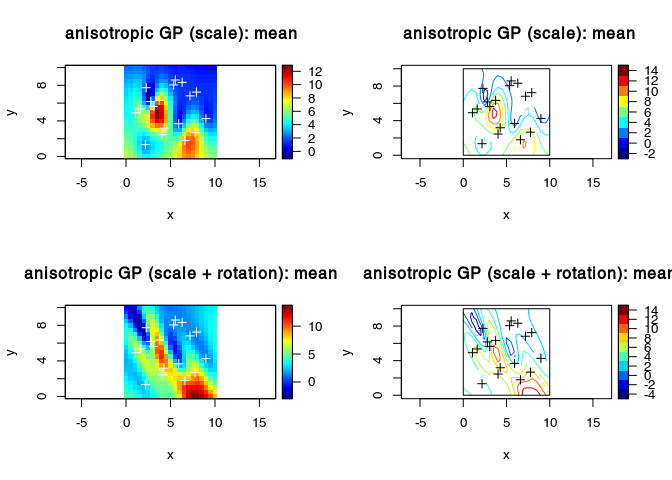
Anisotropy (scaling and rotation along the coordinates axes)
covModelAni2 <- list(kernel="matern",
                 l = 1,       # correlation length
                 v = 2.5,     # smoothness
                 h = 2.45,
                 scale = c(1, 0.25),
                 rot = c(1.0))    # std. deviation
# 2D linear mean function
op <- 2

GP <- gpCond(obs = obs, targ = targ, covModels=list(pos=covModelAni2),
               sigma = sigma, op = op)
names(GP)
# GP$mean   = mean value at location xstar
# GP$cov    = covariance matrix of the conditioned GP
# GP$logLik = log-likelihood of the conditioned GP
# GP$xstar  = x-coordinates at which the GP is simulated
Plot the mean and standard deviation functions
# mean
YmeanAni2 <- matrix(GP$mean, nrow = length(vx), ncol = length(vy), byrow = TRUE)
# standard deviation
YSDAni2 <- matrix(sqrt(diag(GP$cov)), nrow = length(vx), ncol = length(vy),
              byrow = TRUE)

par(mfrow = c(2,2))
plot3D::image2D(x = vx, y = vy, z = YmeanAni, asp = 1)
points(obs$x, col="white",pch=3)
title(main = "anisotropic GP (scale): mean ")

plot3D::contour2D(x = vx, y = vy, YmeanAni, asp = 1)
points(obs$x, col="black",pch=3)
rect(vx[1], vy[1], vx[length(vx)], vy[length(vy)])
title(main = "anisotropic GP (scale): mean")

plot3D::image2D(x = vx, y = vy, z = YmeanAni2, asp = 1)
points(obs$x, col="white",pch=3)
title(main = "anisotropic GP (scale + rotation): mean ")

plot3D::contour2D(x = vx, y = vy, YmeanAni2, asp = 1)
points(obs$x, col="black",pch=3)
rect(vx[1], vy[1], vx[length(vx)], vy[length(vy)])
title(main = "anisotropic GP (scale + rotation): mean")
Gaussian process with derivative constraints
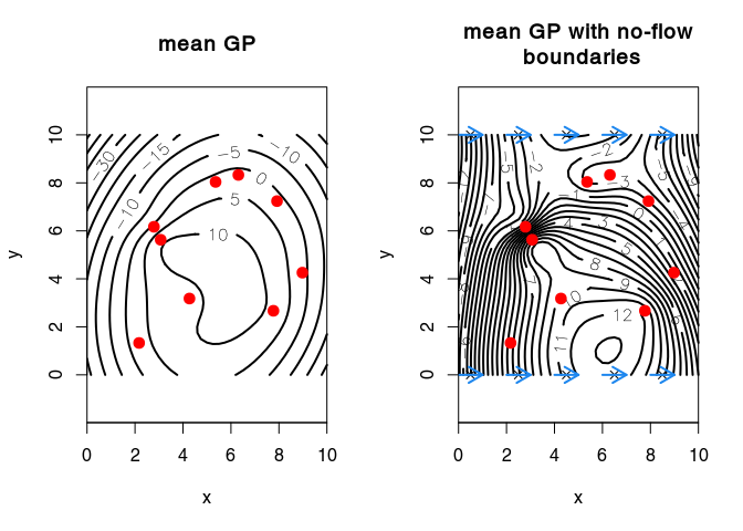
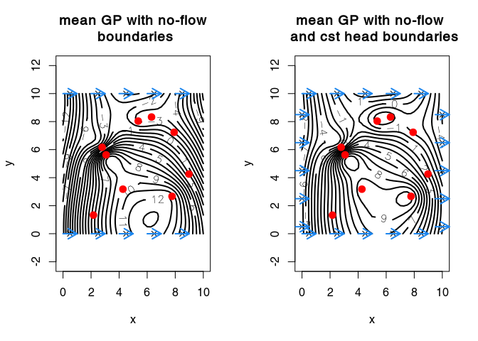
Interpolation of hydraulic heads that accounts for no-flow boundary conditions at the top and bottom model boundary (adapted from Kuhlman and Igúzquiz, 2010, <doi:10.1016/j.jhydrol.2010.01.002>).
We create a new object bc (a list) with elements
xis the locations where we set the derivative of the Gaussian field,vthe gradient derivative, i.e., a unit vector normal to the no-flow boundary (or tangent to a constant-head boundary)yis the value of the gradient (in this case0meaning that the gradient is flat)sigmathe standard deviation reprensenting the uncertainty on the value of the gradient (i.e.,y).
obs <- list(x = cbind(c(2.17, 7.92, 8.98, 7.77, 2.79, 5.36, 4.27, 3.07, 6.31),
                      c(1.33, 7.24, 4.26, 2.67, 6.17, 8.04, 3.18, 5.63, 8.33)),
            y = c(2.60, 1.48, 1.36, 8.61, 1.00, 1.58, 8.42, 8.39, 1.50))


# Matern kernel

vx <- seq(0, 10, by = 0.25)
vy <- seq(0, 10, by = 0.25)
targ <- list(x = vecGrid(vx, vy))


covModel <- list(kernel="matern",
                 l = 1,
                 v = 2.5,
                 h = 3)

op <- 5
sigma <- 0.05


GP <- gpCond(obs = obs, targ = targ, covModels=list(pos=covModel),
             sigma = sigma, op = op)
# mean
Ymean <- matrix(GP$mean, nrow = length(vx), ncol = length(vy), byrow = TRUE)

#  no-flow boundary top and bottom
bc <- list(x = cbind(c( rep(seq(0.5, 9.5, by = 2), 2)),
                     c(rep(0, 5), rep(10, 5))),
           v = cbind( rep(0, 10),
                      rep(1, 10) ),
           y =  rep(0, 10),
           sigma = 0)


GPbc <- gpCond(obs = obs, targ = targ, covModels=list(pos=covModel),
             sigma = sigma, op = op, bc = bc)
# mean
Ymeanbc <- matrix(GPbc$mean, nrow = length(vx), ncol = length(vy), byrow = TRUE)

par(mfrow = c(1,2))


plot3D::contour2D(x = vx, y = vy, Ymean, asp=1, nlevels = 20, col = "black", lwd = 2,
                  xaxs = "i", yaxs = "i", labcex = 1)
points(obs$x, pch=20, col = "red", cex = 2)
#rect(vx[1], vy[1], vx[length(vx)], vy[length(vy)])
title(main = "mean GP")


plot3D::contour2D(x = vx, y = vy, Ymeanbc, asp=1, nlevels = 20, col = "black", lwd = 2,
                  xaxs = "i", yaxs = "i", labcex = 1)
points(obs$x, pch=20, col = "red", cex = 2)
#rect(vx[1], vy[1], vx[length(vx)], vy[length(vy)])
title(main = "mean GP with no-flow\n boundaries")

points(bc$x, pch = 4)
arrows(bc$x[,1] - bc$v[,2]/2, bc$x[,2] - bc$v[,1]/2,
       bc$x[,1] + bc$v[,2]/2, bc$x[,2] + bc$v[,1]/2,
       length = 0.15, col = "dodgerblue2", lwd = 2)
The same with:
- no-flow condition at top and bottom model boundaries
- constant-head boundary at left and right model boundaries
#  no-flow boundary top and bottom
bc2 <- list(x = cbind(c( rep(seq(0.5, 9.5, by = 2), 2),
                        rep(0, 5), rep(10, 5)),
                     c( rep(0, 5), rep(10, 5),
                        rep(seq(0.5, 9.5, by = 2), 2))),
           v = cbind( rep(0, 20),
                      rep(1, 20) ),
           y =  rep(0, 20),
           sigma = 0)

GPbc2 <- gpCond(obs = obs, targ = targ, covModels=list(pos=covModel),
             sigma = sigma, op = op, bc = bc2)
# mean
Ymeanbc2 <- matrix(GPbc2$mean, nrow = length(vx), ncol = length(vy), byrow = TRUE)

par(mfrow = c(1,2))


plot3D::contour2D(x = vx, y = vy, Ymeanbc, asp=1, nlevels = 20, col = "black", lwd = 2,
                  xaxs = "i", yaxs = "i", labcex = 1, xlim = c(-0.5, 10.5))
points(obs$x, pch=20, col = "red", cex = 2)
title(main = "mean GP with no-flow\n boundaries")

points(bc$x, pch = 4)
arrows(bc$x[,1] - bc$v[,2]/2, bc$x[,2] - bc$v[,1]/2,
       bc$x[,1] + bc$v[,2]/2, bc$x[,2] + bc$v[,1]/2,
       length = 0.15, col = "dodgerblue2", lwd = 2)

plot3D::contour2D(x = vx, y = vy, Ymeanbc2, asp=1, nlevels = 20, col = "black", lwd = 2,
                  xaxs = "i", yaxs = "i", labcex = 1, xlim = c(-0.5, 10.5))
points(obs$x, pch=20, col = "red", cex = 2)
title(main = "mean GP with no-flow \n and cst head boundaries")

points(bc2$x, pch = 4)
arrows(bc2$x[,1] - bc2$v[,2]/2, bc2$x[,2] - bc2$v[,1]/2,
       bc2$x[,1] + bc2$v[,2]/2, bc2$x[,2] + bc2$v[,1]/2,
       length = 0.15, col = "dodgerblue2", lwd = 2)
Space-time Gaussian Process Modelling
To understand everything, please read the previous sections.
Observations and target
The observations are defined by a list with x the positions of the observations, y the observed time-series and t the time scale. Note that all the time-series must have the same time scale. Here, the element x of the observation list is a matrix corresponding to the coordinates of the observations points (East/North coordinates or x/y coordinates).
The element y is a big vector constiting of all the time-series recorded at the positions defined by element x put one after another. For example, consider 5 monitoring stations with positions x1, x2, x3, x4 and x5. At each station, a time-series was recorded:
- at station 1: y1 = y1,1, y1,2, …, y1,t
- at station 2: y2 = y2,1, y2,2, …, y2,t
- …
- at station 5: y5 = y5,1, y5,2, …, y5,t
Then, the element y is set to c(y1, y2, y3, y4, y5).
Assuming that the data were recorded every hour, the time scale t is simply 1, 2, 3, …, t.
#observations
obs <- list(x = cbind(c(2, 8, 1, 3, 5),
                      c(9, 2, 3, 4, 6)),
            y = c(1:10 + rnorm(10, 0, 0.1),
                  1:10 + rnorm(10, -0.5, 0.1),
                  1:10 + rnorm(10, 1, 0.4),
                  1:10 + rnorm(10, -0.5, 0.2),
                  1:10 + rnorm(10, 0, 0.1)),
            t = seq_len(10))
The target is defined by a regular grid defined by two orthogonal vectors. The function vecGridreturns a two-columns matrix corresponding to the coordinates of each element of the grid. For each element of the grid, the Gaussian process simulate a time-series whose time scale is identical to that of the observations.
# targets
vx <- seq(0, 10, by = 0.5)
vy <- seq(0, 10, by = 0.5)
targ <- list(x = vecGrid(vx, vy))
Covariance function, mean function and likelihood
Two covariance are defined, one for the space domain (element pos) and one for the time domain (element time). For the moment, the covariance function of the space-time Gaussian process is defined by the product of the spatial and temporal kernel.
covModels <- list(pos =  list(kernel="matern",
                              l = 4,       # correlation length
                              v = 2.5,     # smoothness
                              h = 2.45),    # std. deviation
                  time = list(kernel="gaussian",
                              l = 0.15,   # correlation length
                              h = 1.25))

# 2D mean linear mean function
op <- 2

# Gaussian likelihood
sigma <- 0.2
Conditional Gaussian Process modelling
GP <- gpCond(obs = obs, targ = targ, covModels = covModels,
               sigma = sigma, op = op)
names(GP)
# GP$mean   = mean value at location xstar
# GP$cov    = covariance matrix of the conditioned GP
# GP$logLik = log-likelihood of the conditioned GP
# GP$xstar  = x-coordinates at which the GP is simulated
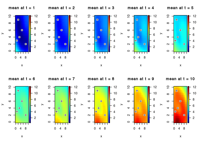
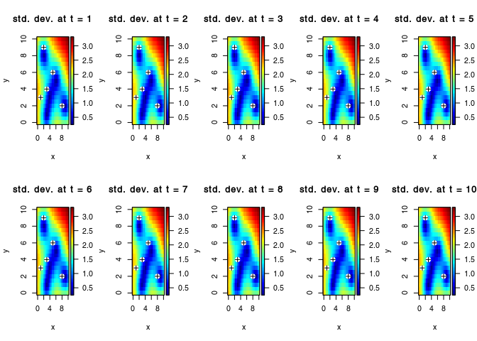
The mean values are re-organised into a three-dimensional array of dimension $n_t n_x n_y, with nt the number of time-step, and nx × ny the dimension of the (spatial) target grid.
Ymean <-  array(GP$mean, dim=c(length(obs$t), length(vx), length(vy)))
Ysd <-  array(sqrt(diag(GP$cov)), dim=c(length(obs$t), length(vx), length(vy)))

par(mfrow = c(2,5))
for(i in seq_along(obs$t)){
  plot3D::image2D(z = Ymean[i,,], x = vx, y = vy, zlim = range(Ymean),
                  main = paste("mean at t =",obs$t[i]))
  points(obs$x, col="white",pch=20, cex=2)
  points(obs$x, col="black",pch=3)
}
par(mfrow = c(2,5))
for(i in seq_along(obs$t)){
  plot3D::image2D(z = Ysd[i,,], x = vx, y = vy, zlim = range(Ysd),
                  main =  paste("std. dev. at t =",obs$t[i]))
  points(obs$x, col="white",pch=20, cex=2)
  points(obs$x, col="black",pch=3)
}
Random conditional simulation. La function gpSim returns a matrix whose two first column correspond to the position coordinate, the third columns corresponds to the time scale and the fourth column to the simulated Gaussian process.
L <- cholfac(GP$cov)
ystar <- gpSim(GP , L = L)

colnames(ystar) <- c("x1", "x2", "t", "y")

Ysim <- array(ystar[,"y"], dim=c(length(obs$t), length(vx), length(vy)))

par(mfrow = c(2,5))
for(i in seq_along(obs$t)){
  plot3D::image2D(z = Ysim[i,,], x = vx, y = vy,
                  zlim = range(ystar[,"y"]),
                  main = paste("simulation at t =",obs$t[i]))
  points(obs$x, col="white",pch=20, cex=2)
  points(obs$x, col="black",pch=3)
}

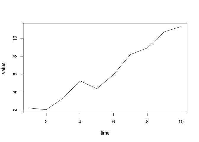
Time-series at location (4,1):
par(mfrow = c(1,1))
plot(Ysim[,vx == 4, vy == 1], type = "l", xlab = "time", ylab = "value")
References
Rasmussen C.E. and Williams C.K.I. (2006), Gaussian Processes for Machine Learning, the MIT Press, ISBN 026218253X. www.GaussianProcess.org/gpml