Note:
RGPR# install "devtools" if not already done
if(!require("devtools")) install.packages("devtools")
devtools::install_github("emanuelhuber/RGPR")
## labeling    (0.4.2   -> 0.4.3) [CRAN]
## htmltools   (0.5.5   -> 0.5.6) [CRAN]
## cpp11       (0.4.5   -> 0.4.6) [CRAN]
## purrr       (1.0.1   -> 1.0.2) [CRAN]
## dplyr       (1.1.2   -> 1.1.3) [CRAN]
## tinytex     (0.45    -> 0.46) [CRAN]
## fontawesome (0.5.1   -> 0.5.2) [CRAN]
## bslib       (0.5.0   -> 0.5.1) [CRAN]
## xfun        (0.39    -> 0.40) [CRAN]
## rmarkdown   (2.23    -> 2.25) [CRAN]
## knitr       (1.43    -> 1.44) [CRAN]
## askpass     (1.1     -> 1.2.0) [CRAN]
## curl        (5.0.1   -> 5.0.2) [CRAN]
## gtable      (0.3.3   -> 0.3.4) [CRAN]
## DEoptimR    (1.1-0   -> 1.1-2) [CRAN]
## wk          (0.7.3   -> 0.8.0) [CRAN]
## promises    (1.2.0.1 -> 1.2.1) [CRAN]
## httr        (1.4.6   -> 1.4.7) [CRAN]
## ggplot2     (3.4.2   -> 3.4.3) [CRAN]
## units       (0.8-2   -> 0.8-4) [CRAN]
## classInt    (0.4-9   -> 0.4-10) [CRAN]
## terra       (1.7-39  -> 1.7-46) [CRAN]
## fields      (14.1    -> 15.2) [CRAN]
## adimpro     (0.9.5   -> 0.9.6) [CRAN]
## Cairo       (1.6-0   -> 1.6-1) [CRAN]
## ── R CMD build ─────────────────────────────────────────────────────────────────
##      checking for file ‘/tmp/RtmpzyfoS1/remotes46ab2ebd7edb/emanuelhuber-RGPR-0ba96b9/DESCRIPTION’...  ✔  checking for file ‘/tmp/RtmpzyfoS1/remotes46ab2ebd7edb/emanuelhuber-RGPR-0ba96b9/DESCRIPTION’
##   ─  preparing ‘RGPR’:
## ✔  checking DESCRIPTION meta-information
##   ─  checking for LF line-endings in source and make files and shell scripts
##   ─  checking for empty or unneeded directories
##        NB: this package now depends on R (>= 3.5.0)
##        WARNING: Added dependency on R >= 3.5.0 because serialized objects in
##      serialize/load version 3 cannot be read in older versions of R.
##      File(s) containing such objects:
##        ‘RGPR/test.rds’
##   ─  building ‘RGPR_0.0.7.tar.gz’
##
##
library(RGPR) # load RGPR in the current R session
RPGR comes along with a GPR data called frenkeLine00. Because this
name is long, we set A equal to frenkeLine00:
x <- frenkeLine00
x
## *** Class GPR ***
##  name        = LINE00
##  filepath    = data-raw/LINE00.DT1
##  1 fiducial(s)
##  description =
##  survey date = 2014-04-25
##  Reflection, 100 MHz, Window length = 399.6 ns, dz = 0.4 ns
##  223 traces, 55.5 m
##  ****************
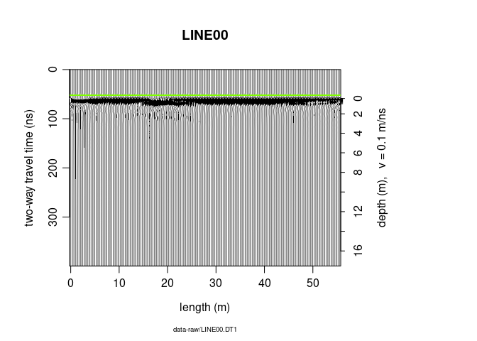
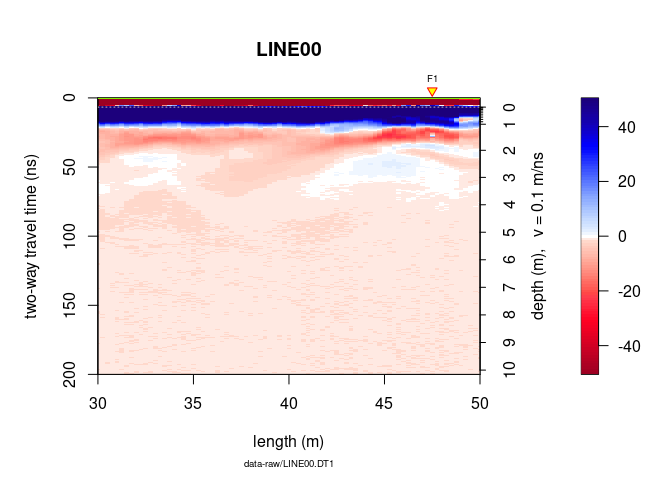
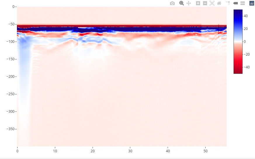
To plot the GPR record as a raster image (default mode), enter
plot(x)
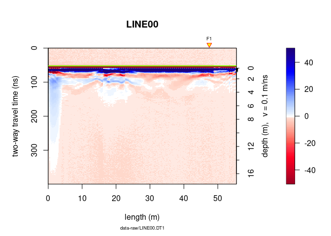
The green line indicates the position of time-zero. The yellow triangle indicates the position of a fiducial marker that was set during the survey to mark something (such as a specific object close to the GPR line, a change in morphology/topography/sedimentology or an intersection with another GPR line). These markers are very useful to add topographic data to the GPR profile, particularly when the fiducial markers correspond to the locations where the (x,y,z) coordinates were measured.
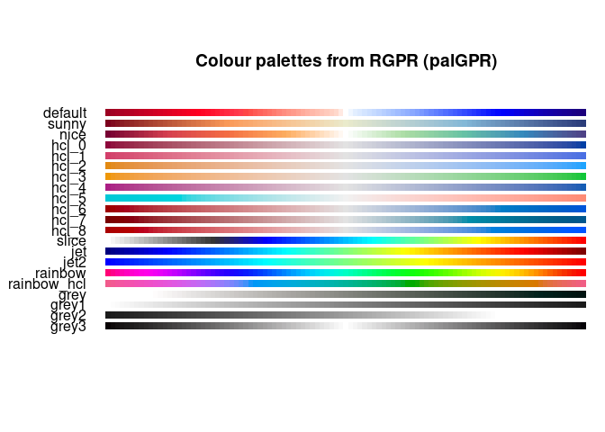
Do you want another color palette? RGPR comes with predefined color palettes. Check them with:
displayPalGPR()
Plot a single palette:
plotPal(palGPR("nice"))

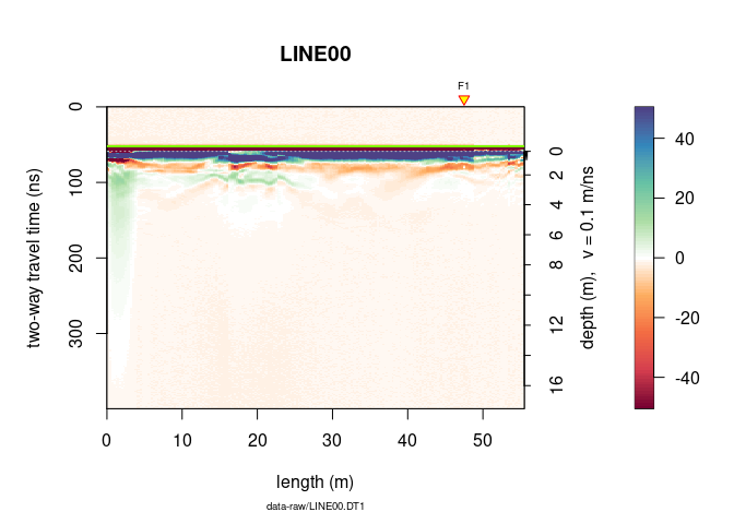
Choose the color palette you want and plot the GPR data with it:
plot(x, col = palGPR("nice"))
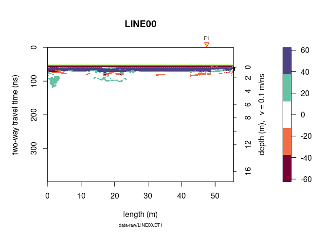
You can reduce the number of colors with:
plot(x, col = palGPR("nice", n = 5))
Instead of plot(x) use plotFast(x)!
Plot wiggles
plot(x, type = "wiggles")
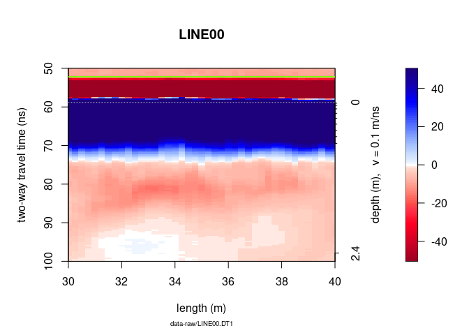
To plot only a part of the GPR data, use xlim and ylim.
plot(x, ylim = c(50, 100), xlim = c(30, 40))
Another way to plot only a part of the GPR data is to extract a part of
the GPR data. The object A can be manipulated in the same way as a
matrix without losing the meta-data (e.g., trace coordinates, antenna
separation).
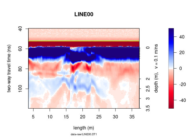
To plot only the samples 100 to 300 of the $15^{th}$ to $150^{th}$ :
# plot the 100 to 300 samples of the traces 15 to 150
plot(x[100:300, 15:150])
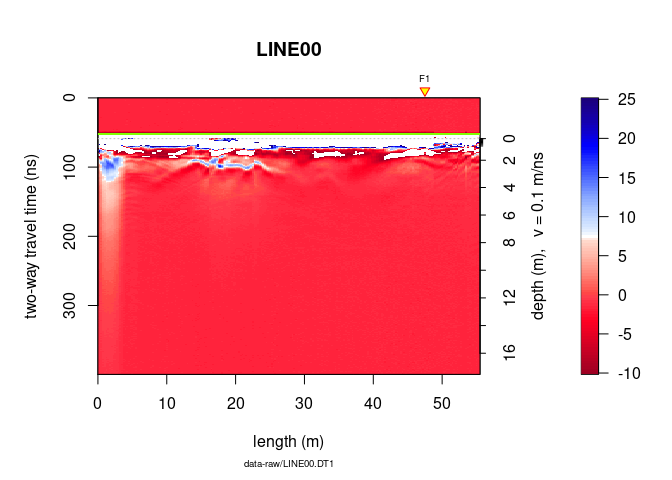
To change the span of the colorbar from -10 to 25 do
plot(x, zlim = c(-10, 25))
To set the origin of the vertical axis at time-zero, set the argument
relTime0 equal to TRUE.
plot(x, relTime0 = TRUE, ylim = c(0, 200), xlim = c(30, 50))
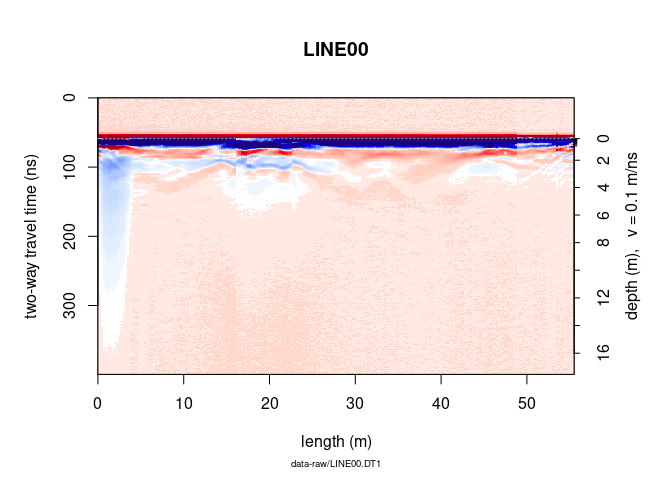
To not display the markers, the annotation (e.g., markers for the
intersection of the GPR line with other GPR lines), the time-zero line,
the colorbar (barscale), set addFid, addAnn, addTime0 and
barscale equal to FALSE.
plot(x, addFid = FALSE, addAnn = FALSE, addTime0 = FALSE, barscale = FALSE)
To not display the note below the x-label, the plot title (file name),
the x and y lables, the colorbar label, set note, main, ylab,
xlab and clab equal to "".
plot(x, note = "", main = "", ylab = "", xlab = "", clab = "")
ggplot2 plotsPlots with ggplot2, a R-package based on the Grammar of Graphics.
x <-frenkeLine00

ggplotGPR(x)
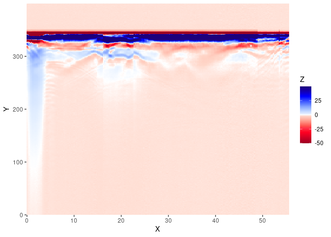
The ggplotGPR() function is a wrapper for:
col <- palGPR()
x <- frenkeLine00

Xm <- data.frame(x = rep(pos(x), nrow(x)),
                 y = rep(depth(x), each = ncol(x)),
                 value =  as.vector(t(as.matrix(x)[nrow(x):1, ])))
ggplot2::ggplot(Xm) +
  ggplot2::geom_tile(ggplot2::aes(x = x, y = y, fill = value)) +
  ggplot2::scale_x_continuous("X", expand = c(0, 0)) +
  ggplot2::scale_y_continuous("Y", expand = c(0, 0)) +
  ggplot2::scale_fill_gradientn("Z", colours = col)
Use the function plotly() to produce interactive plots powered powered
by the JavaScript library plotly.js. The function plotly() works only
with 2D data.
x <- frenkeLine00

plotly(x)
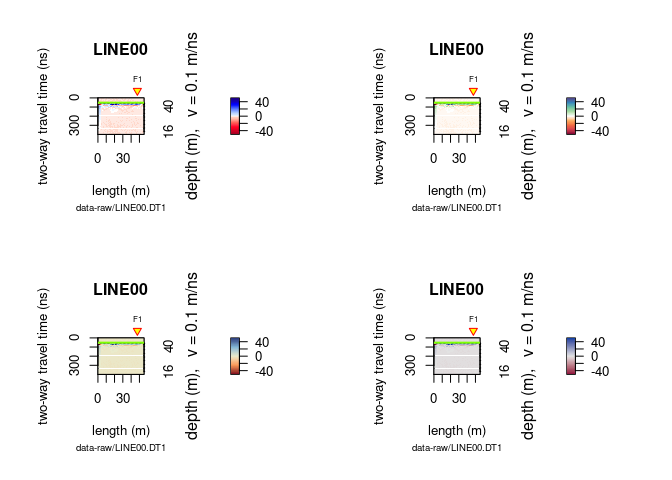
Use par(mfrow = c(nr, nc)), where ncr is the number of rows and nc
is the number of column. Example:
x <- frenkeLine00

par(mfrow = c(2,2), oma = c(0, 0, 0, 0))
plot(x)
plot(x, col = palGPR("nice"))
plot(x, col = palGPR("sunny"))
plot(x, col = palGPR("hcl_0"))
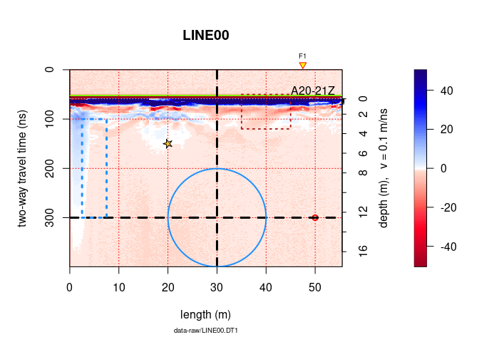
Here an example on how to annotate plots:
x <- frenkeLine00

plot(x)
rect(xleft = 35,
     ybottom = 120,
     xright = 45,
     ytop = 50,
     border = "firebrick",
     lty = 3,   # line style: 1 = continuous line
     lwd = 2)   # width
# text annotation
text(45, 50, "A20-21Z", adj = c(0, 0))
#grid
grid(col = "red")
# point
points(50, 300, pch = 21, col = "red", lwd = 2)
# horizontal and vertical linges
abline(h = 300, v = 30, col = "black", lty = 2, lwd = 3)

# For circles, squares and stars the units of the x axis are used
# circles
symbols(30, 300, circles = 10,
        add = TRUE, lwd = 2, fg = "dodgerblue", inches = FALSE, lty = 1)
# rectangles
symbols(5, 200, rectangles = matrix(c(5, 200), nrow = 1, ncol = 2),
        add = TRUE, lwd = 3, fg = "dodgerblue", inches = FALSE, lty = 3)
# stars
symbols(20, 150, stars = matrix(c(0.35, 1, 0.35, 1,  0.35, 1,  0.35, 1, 0.35, 1), nrow = 1),
        add = TRUE, lwd = 1, bg = "goldenrod1", fg = "black", inches = FALSE, lty = 1)
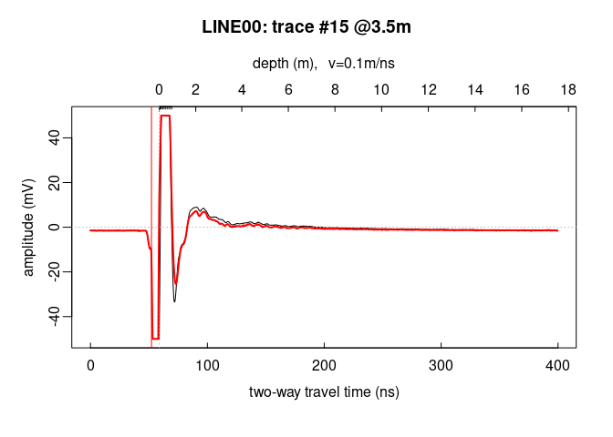
Plot a signal trace, notice that the signal is clipped to $\pm50\,mV$ (between $0$ and $20\,ns$ ):
plot(x[, 15]) # plot the 15th trace of the GPR-line
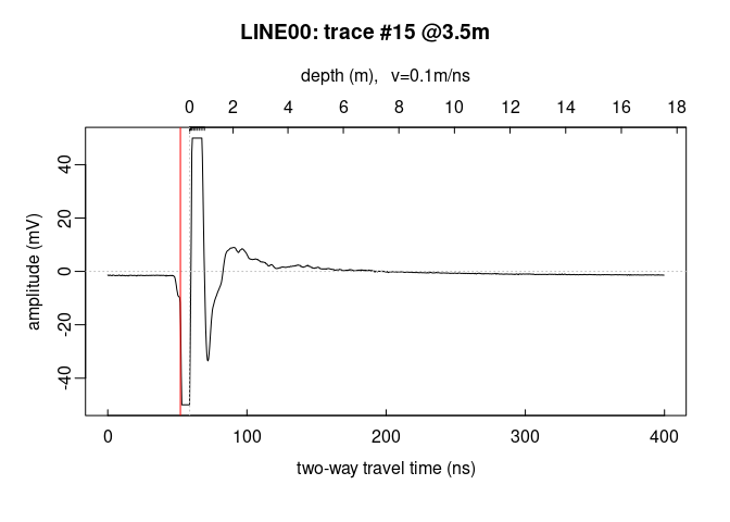
Note: the @3.5m in the plot title indicate the relative position of
the trace on the GPR profile.
To add another trace, use the function lines()
plot(x[, 15])      # plot the 15th trace of the GPR-line
lines(x[, 16], col = "red", lwd = 2)
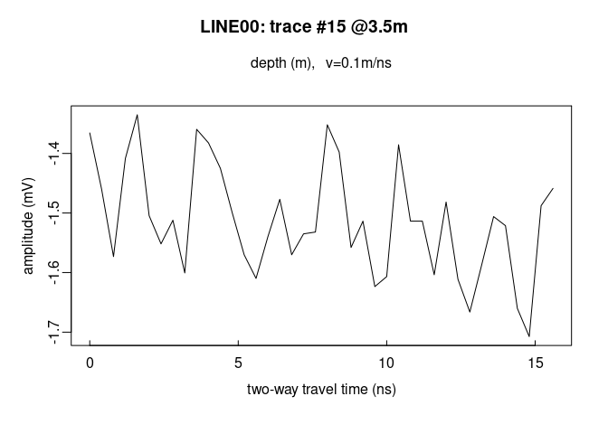
Plot the first 40 trace samples:
# plot the first 40 samples of the 15th trace of the GPR profile
plot(x[1:40, 15])
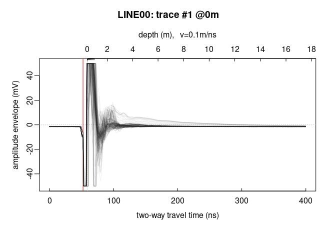
Plot all the traces within a single plot:
trPlot(x, col = rgb(0.2, 0.2, 0.2, 7/100)) # plot all the traces
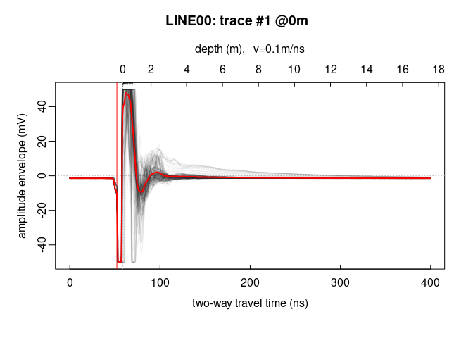
Add the average trace
trPlot(x, col = rgb(0.2, 0.2, 0.2, 7/100))     # plot all the traces
lines(traceStat(x), lwd = "2", col = "red")
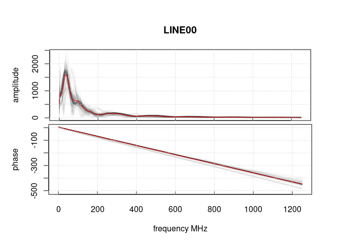
Let’s have a look at the amplitude-frequency and phase-frequency plot (the spectrum given by the Fourier decomposition):
spec(x)
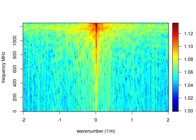
The function spec() with the argument type = "f-k returns a list
containing the frequencies (f), the wavenumbers (k), the amplitude of
the GPR data.
spec(x, type = "f-k")
Check the help for more details on the plot() function:
?plot.GPR
?trPlot