Hyperbola fitting

Note:

• This R-package is still in development, and therefore some of the functions may change in a near future.
• If you have any questions, comments or suggestions, feel free to contact me (in english, french or german): emanuel.huber@pm.me.

Table of Contents

• Objectives of this tutorial
• Preliminary
  • Install/load RGPR
  • The GPR data
  • Basic processing
• Hyperbola fitting
  • Interactive point selection and hyperbola fitting
  • Plot the fitted hyperbola
  • Plot an hyperbola defined by its vertex position and the root-mean-square velocity
  • Simulate an hyperbola

Objectives of this tutorial

• Learn how to fit manually a hyperbola to GPR data

Note that his tutorial will not explain you the math/algorithms behind the different processing methods.

Preliminary

• Read the tutorial Basic GPR data processing to learn more about the processing methods

Install/load RGPR

# install "devtools" if not already done
if(!require("devtools")) install.packages("devtools")
devtools::install_github("emanuelhuber/RGPR")
library(RGPR)       # load RGPR in the current R session

The GPR data

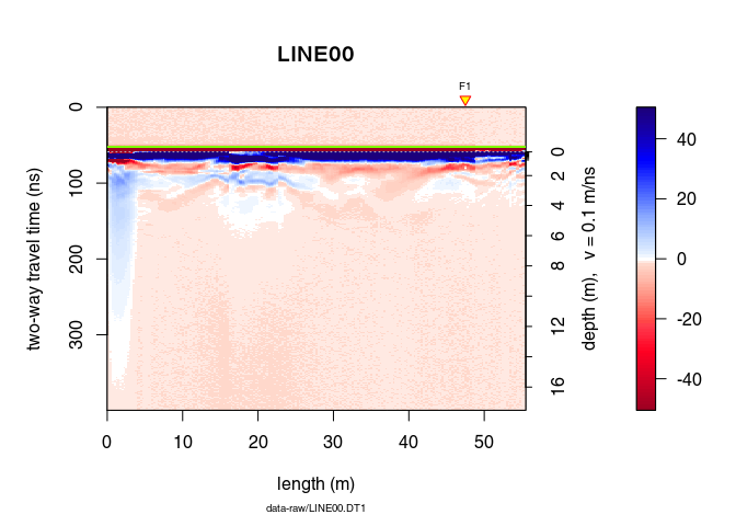
RPGR comes along with a GPR data called frenkeLine00. Because this name is long, we set x equal to frenkeLine00:

x <- frenkeLine00
plot(x)

Basic processing

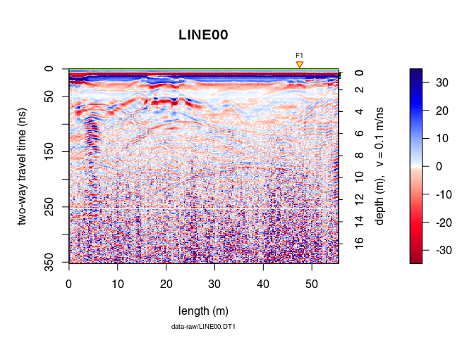
We apply some basic processing to the data with the pipe operator (%>%):

x <- x %>%  estimateTime0(w = 5, method = "MER", FUN = mean) %>%
     time0Cor(method = "pchip")  %>%
     dewow(type = "Gaussian", w = 5)  %>%
     fFilter(f = c(200, 300), type = "low") %>%
     gainSEC(a = 0.003, t0 = 50)

plot(x)

Hyperbola fitting

Interactive point selection and hyperbola fitting

Select points interactively on the plot with

xy <- locator(type = "l")

## $x
## [1] 11.8 15.0 17.7 20.3 24.4 27.4 30.9 35.2
##
## $y
## [1] 142.2 119.8 107.7  99.5  97.5 105.6 120.9 138.1

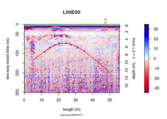
Fit the corresponding hyperbola with the function hyperbolaFit():

hyp <- hyperbolaFit(xy)

hyperbolaFit() returns:

• the hyperbola vertex: c(hyp$x0, hyp$t0)
• the estimated root-mean-square velocity: hyp$vrms
• the estimated depth of the hyperbola vertex (computed using the root-mean-square velocity): hyp$z0
• the input points for the fitting: hyp$xand hyp$y
• the output of the regression fit (see R function lm()): hyp$reg

Plot the fitted hyperbola

• Plot the hyperbola for x-position ranging from 5 to 50:

  plot(x)
  points(xy, pch = 20, col = "blue")
  hyperbolaPlot(hyp, x = seq(5, 50, by = 0.01), col = "red", lwd = 2)
  

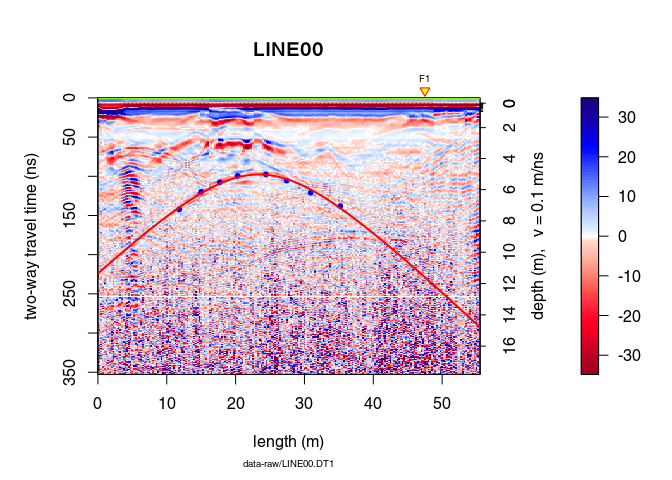
• Plot the hyperbola without defining its x-position (in this case the hyperbola is displayed over the entire plot)

  plot(x)
  points(xy, pch = 20, col = "blue")
  hyperbolaPlot(hyp, col = "red", lwd = 2)
  

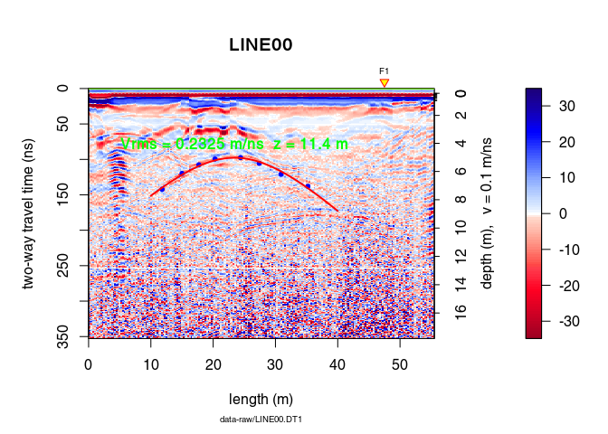
• Define the hyperbola range with xlim and add some annotations:

  plot(x)
  points(xy, pch = 20, col = "blue")
  hyperbolaPlot(hyp, col = "red", lwd = 2, xlim = c(10, 40), ann = TRUE)
  

Plot an hyperbola defined by its vertex position and the root-mean-square velocity

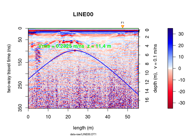
Define the hyperbola parameters

hyp2 <- list(x0 = hyp$x0, t0 = hyp$t0, vrms = hyp$vrms)

Plot the hyperbola

plot(x)
points(hyp$x0, hyp$t0, pch = 20, col = "red", cex = 1.3)
hyperbolaPlot(hyp2, col = "blue", lwd = 2, ann = TRUE)

Simulate an hyperbola

• Using the output of hyperbolaFit():

  xv <- seq(5, 45, by = 0.1)
  y <- hyperbolaSim(xv, hyp)
  plot(x)
  points(hyp$x0, hyp$t0, pch = 20, col = "blue")
  lines(xv, y)
  

• Defining its vertex position and the root-mean-square velocity:

  hyp2 <- list(x0 = hyp$x0, t0 = hyp$t0, vrms = hyp$vrms)
  xv <- seq(5, 45, by = 0.1)
  y <- hyperbolaSim(xv, hyp2)
  plot(x)
  lines(xv, y)
  points(hyp$x0, hyp$t0, pch = 20, col = "blue")