-– layout: page title: GPR data migration date: 2023-09-24 -–

Note:

• This R-package is still in development, and therefore some of the functions may change in a near future.
• If you have any questions, comments or suggestions, feel free to contact me (in english, french or german): emanuel.huber@pm.me.

Table of Contents

• Objectives of this tutorial
• Preliminary
  • File organisation
  • Install/load RGPR and set the working directory
• Read GPR data
• Pre-processing
  • Add topographic data (coordinates)
  • DC shift removal
  • First wave break estimation and set time-zero
  • Dewow
  • Frequency filter
  • Time gain
• Topographic Kirchhoff migration
  • Pre-processing
    • Constant offset correction
    • Time upsampling (sinc-interpolation) of the GPR data to reduce the aliasing risk.
  • Topographic Kirchhoff migration.
  • Post-processing
  • Comparison before/after migration

Objectives of this tutorial

Learn how to migrate GPR data.

Note that his tutorial will not explain you the math/algorithms behind the different processing methods.

Preliminary

• Download the data 2014_04_25_frenke.zip
• Unzip the data

File organisation

I suggest to organise your files and directories as follows:

/2014_04_25_frenke   (project directory with date and location)
    /processing      (here you will save the processed GPR files)
    /rawGPR          (the raw GPR data, never modify them!)
    RGPR_tutorial.R  (this is you R script for this tutorial)

Install/load RGPR and set the working directory

• Install and load the RGPR-package

  # install "devtools" if not already done
  if(!require("devtools")) install.packages("devtools")
  devtools::install_github("emanuelhuber/RGPR")
  library(RGPR)       # load RGPR in the current R session
  

• Set the working directory:

  myDir <- "~/2014_04_25_frenke"  # adapt that to your directory structure
  setwd(myDir)    # set the working directory
  getwd()         # Return the current working directory (just to check)
  

Read GPR data

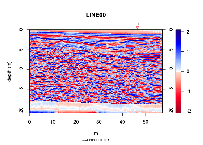
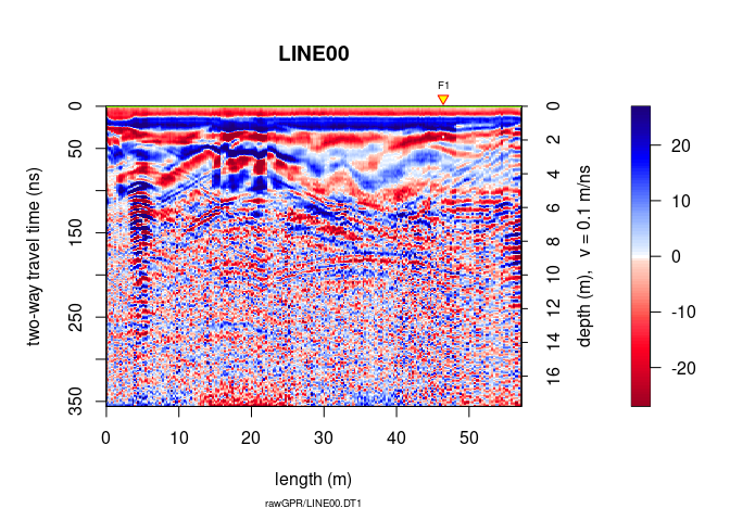
A <- readGPR(fPath = "rawGPR/LINE00.DT1")   # the filepath is case sensitive!

## Warning in readGPR(fPath = "rawGPR/LINE00.DT1"): Argument 'fPath' is
## deprecated. Use instead 'dsn' (data source name)

Pre-processing

Add topographic data (coordinates)

We assume that for each GPR record there is a file containing the (x, y, z) coordinates of every traces. The header of these files is “E”, “N”, “Z” instead of “x”, “y”, “z” because in topography “x” sometimes designates the North (“N”) and not the East (“E”) as we would expect. The designation “E”, “N”, “Z” is less prone to confusion and therefore we chose it!

1. Define the filepaths to the topo files:

TOPO <- file.path(getwd(), "coord/topo/LINE00.txt")

1. Read all the files with the funciton readTopo() that creates a list whose elements correspond to the GPR record and contain all the trace coordinates:

TOPOList <- readTopo(TOPO, sep = "\t")

## read /mnt/data/Documents/RESEARCH/PROJECTS/RGPR/CODE/RGPR-gh-pages/2014_04_25_frenke/coord/topo/LINE00.txt...

1. Set the list of coordinates as the new coordinates to the GPRsurvey object:

coord(A) <- TOPOList[[1]]

DC shift removal

Remove the DC-offset estimated on the first n samples usind the function dcshift(). This function takes as argument the GPR object and the sample index used to estimate the DC shift (in this case, the first 110 samples):

A1 <- dcshift(A, 1:110)   # new object A1

First wave break estimation and set time-zero

The first wave break time, t_fb, is estimated for each traces

tfb <- firstBreak(A1, w = 20, method = "coppens")   # take some time

Convert the first wave break time t_fb into time-zero t₀ with firstBreakToTime0().

Here we define $t_0 = t_{\text{fb}} -\frac{a}{c_0}$, where a is the distance between the transmitter and receiver and c₀ is the wave velocity in the media between the transmitter and receiver (in our case, air). The value $\frac{a}{c_0}$ corresponds to the wave travel time from the transmitter to the receiver.

t0 <- firstBreakToTime0(tfb, A1)
time0(A1) <- t0     # set time0 to A1

To shift the traces to time-zero, use the function time0Cor.

A2 <- time0Cor(A1, method = "spline")

Dewow

Remove the low-frequency components (the so-called “wow”) of the GPR record with:

A3 <- dewow(A2, type = "runmed", w = 50)

Frequency filter

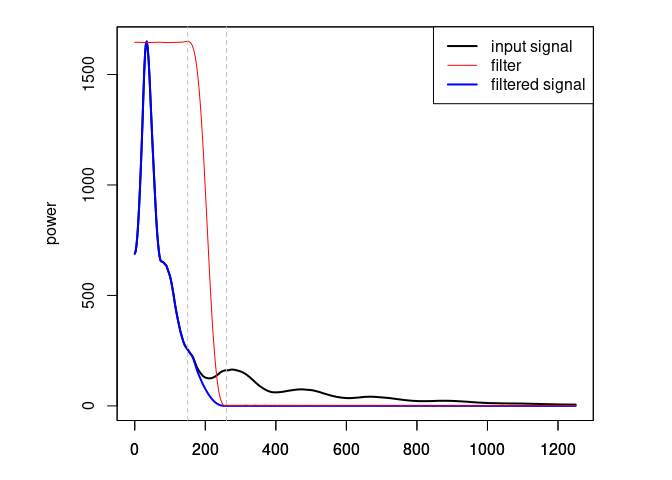
Eliminate the high-frequency (noise) component of the GPR record with a bandpass filter. We define as corner frequencies at 150 MHz and 260 MHz, and set plotSpec = TRUE to plot the spectrum with the signal, the filtered signal and the filter.

A4 <- fFilter(A3, f = c(150, 260), type = "low", plotSpec = TRUE)

Time gain

Apply a power gain and a spherical gain to compensate for geometric wave spreading and attenuation (Kruse and Jol, 2003; Grimm et al., 2006).

A5 <- gain(A4, type = "power", alpha = 1, te = 150, tcst = 20)
A6 <- gain(A5, type = "exp", alpha = 0.11, t0 = 0, te = 125)

Topographic Kirchhoff migration

See Dujardin & Bano (2013, Topographic migration of GPR data: Examples from Chad and Mongolia, Comptes Rendus Géoscience, 345(2):73-80. Doi: 10.1016/j.crte.2013.01.003)

Pre-processing

Constant offset correction

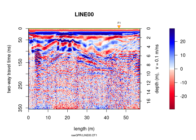
Time correction for each trace to compensate the offset between transmitter and receiver antennae (it converts the trace time of the data acquired with a bistatic antenna system into trace time data virtually acquiered with a monostatic system)

A7 <- timeCorOffset(A6)
plot(A7)

Time upsampling (sinc-interpolation) of the GPR data to reduce the aliasing risk.

A8 <- upsample(A7, n = c(3,1))

Topographic Kirchhoff migration.

Vertical resolution of the migrated data, we set dz = 0.01m.

The dominant return frequency can be estimated by visual inspection of the spectrum of A8 (to display the frequency spectrum of A8 use the function spec(), e.g. spec(A8)). Here, the dominant return frequency is estimated to be $80 MHz$ and therefore we set fdo = 80 (the dominant frequency is used to estimate the Fresnel zone).

For the moment the algorithm works only with a constant radar wave velocity. In this example the velocity is:

vel(A8)         # velocity

## $v
## [1] 0.1

depthunit(A8)   # units: nano-second (ns)

## [1] "ns"

To change the velocity, simply do:

vel(A8)  <- 0.09        # velocity in ns

A9 <- migrate(A8, type="kirchhoff", max_depth = 20,
                 dz = 0.01, fdo = 80)
plot(A9)

You don’t see so much: we need some post-processing!

Post-processing

Trace smoothing with a Gaussian filter

A10 <- filter1D(A9, type = "Gaussian", w = 2.5)

Automatic gain control

A11 <- gain(A10, type = "agc", w = 0.55)

inverse normal transformations

A12 <- traceScaling(A11, type = "invNormal")

Comparison before/after migration

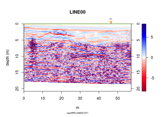
Before migration

plot(traceScaling(A8, type = "invNormal"))

After migration

plot(A12)